Forecasting data design: stations, models, formats and direct access
Print edition: download the full report as a PDF (US Letter, typeset for high-quality printing, with vector figures, a table of contents and lists of figures and tables).
← Back to Forecasts and Model Checks
Weather project, forecasting subproject. Design report, version of 2026-10-27. Measurements marked measured were taken on lamp, the small Linux server that runs the project, on 2026-10-26 and 2026-10-27.
Abstract
This report explains where the numbers on the forecasting page come from and how they are stored. A household in Cumberland Center, Maine, compares free weather forecasts from the National Oceanic and Atmospheric Administration (NOAA) with what its own and nearby weather stations measured, checks whether the stations are still accurate, estimates solar production and forecasts two weeks of heating cost. The model data is read in cloud-native formats, which let a program fetch just the small piece it needs instead of downloading whole files. Reading one year of hourly temperature at the house took 19.3 megabytes (MB) and one second, against roughly 9 gigabytes (GB) in NOAA's traditional files. Checking the stations against two independent references found that the house station has drifted about 2 degrees Fahrenheit (degF) colder since December 2025, and that one volunteer station (E4229) records missing readings as zeros, so it was removed from all analyses. Every forecast is checked against what actually happened. Solar production forecast for tomorrow missed by 7 kilowatt-hours (kWh) on a typical 47 kWh day, against 17 kWh for the normal, and was clearly better than the normal for 5 days. A gas bill forecast a month ahead missed by 24% on average, barely worse than the 22% with the weather already known, so the gas usage model, not the weather forecast, limits it. Household electricity use depends more on habits than on weather: the forecast for tomorrow missed by 7.6 kWh of a typical 42 kWh day, and most of its advantage over the normal comes from tracking the household's recent level of use. The report closes with the one open design decision: keep reading the data through its publisher's helper library, or write our own access code. It recommends keeping the helper library until a concrete reason to switch appears.
Data: six weather stations (five analysed); the NOAA High-Resolution Rapid Refresh (HRRR) analysis and forecasts, the Global Forecast System (GFS) and the 31-member Global Ensemble Forecast System (GEFS) via dynamical.org (SpatioTemporal Asset Catalog (STAC), Icechunk, Zarr v3, virtual GRIdded Binary edition 2 (GRIB2)); and daily grids from the Parameter-elevation Regressions on Independent Slopes Model (PRISM), stored as Cloud Optimized GeoTIFF. Storage: a local Icechunk cube (layer 1, L1), Hive-partitioned Parquet point tables (layer 2, L2) and DuckDB views with MariaDB attached read-only (layer 3, L3). Results: a point-year read of 19.3 MB in 1.0 s against about 9 GB and 17,520 requests by the GRIB2 route; a house-station (ZASTMET) offset change of about -2 degF against the HRRR analysis from December 2025 while the Portland International Jetport station (KPWM) held steady; E4229 excluded for placeholder zeros and a warm bias. Forecast checks against baselines (persistence, 1991-2020 normals): solar production mean absolute error (MAE) 7.0 kWh/day at lead day 1 (normal 16.9, known-weather floor 4.3), skill over the normal clearly (95% bootstrap interval above zero) to day 5, on average to day 7; GEFS weekly heating degree day (HDD) MAE 10 (normal 27), coverage of the calibrated 10th to 90th percentile range (p10-p90) 81%; gas bills replayed from GEFS runs 0-35 days before the meter read, MAE 22% at lead 0 rising to 24% at 29-35 days (normal 29%); household electricity from a change-point model with a 28-day recent level, day-1 MAE 7.6 kWh (normal 9.5, known weather 7.5), weekly total MAE 12%, 80% range coverage 83%; net grid use beats the normal clearly to day 4, on average to day 5. Decision D7: stay on dynamical-catalog; switching costs about 15 hours and changes no stored value.
Keywords: cloud-native data, Zarr, Icechunk, Parquet, STAC, Cloud Optimized GeoTIFF, GRIB2, numerical weather prediction, ensemble forecast, forecast verification, solar production forecast, station quality control, heating degree days.
How to read this report
The report is written for several audiences at once. Each section starts with In plain terms, for readers who are not developers or scientists, followed by For developers, with the technical detail. Terms are explained where they first appear, and Appendix B collects every term and acronym with a link to more information. Click any figure to open it full size. The list below links to every figure, table and code listing.
List of figures, tables and listings
Figures
- Figure 1. Data sources, the lamp server and the analyses on the two forecasting pages
- Figure 2. Station records held in the weather database, 2017 to 2026
- Figure 3. How station readings reach the project's database
- Figure 4. From observations to analyses, forecasts, ensembles and PRISM maps
- Figure 5. Traditional download-then-search versus cloud-native look-up-then-fetch
- Figure 6. One NetCDF/HDF5 file versus a Zarr store of separately addressed objects
- Figure 7. The six data formats and how they relate
- Figure 8. Structure of the dynamical.org STAC catalog
- Figure 9. Structure of an Icechunk repository
- Figure 10. How chunk shape decides which questions are fast
- Figure 11. Shards, inner chunks and codecs of the HRRR temperature array
- Figure 12. Sequence of a cloud-native read through xarray, Zarr and Icechunk
- Figure 13. A GRIB2 file, the sections of one message, and the references that point into it
- Figure 14. Row layout versus column layout of the same readings
- Figure 15. Partition folders and internal structure of one L2 Parquet file
- Figure 16. Plain GeoTIFF versus Cloud Optimized GeoTIFF file layout
- Figure 17. Contents of a PRISM daily download
- Figure 18. The daily data pipeline on lamp
- Figure 19. Library stack from the project's code down to storage
- Figure 20. Write path of one update run: L1 cube, then L2 tables
- Figure 21. Splitting a forecast's error into the usage-model part and the weather-forecast part
- Figure 22. How the wrapper opens a dataset
- Figure 23. How a direct client would open a dataset
- Figure 24. ZASTMET minus the HRRR analysis, monthly mean, January 2024 to October 2026
- Figure 25. One year, one point, one variable: traditional versus cloud-native access
- Figure 26. Virtues of the direct approach
- Figure 27. Downsides of the direct approach
- Figure 28. Effort against learning value of the access options
- Figure 29. Effort to switch to direct access, by task
- Figure 30. Illustrative migration schedule if the decision is reopened
- Figure 31. Decision flow: when to revisit the wrapper
Tables
- Table 1. Analyses on the Forecasts and Model Checks page
- Table 2. The weather stations
- Table 3. Weather models and map products used
- Table 4. dynamical.org datasets read, with dimensions, steps and variables
- Table 5. Main ideas of cloud-native formats and their traditional counterparts
- Table 6. Traditional formats and the cloud-native formats that replace them here
- Table 7. The six formats: role, reader library, and whether the project writes them
- Table 8. Fields of a dynamical.org STAC Collection (HRRR analysis)
- Table 9. Sections of a GRIB2 message
- Table 10. Libraries and the formats they handle
- Table 11. The forecast checks: what is forecast, what it is checked against, and the baselines it must beat
- Table 12. What the wrapper does at each step
- Table 13. Direct access for each piece, with the checks to add
- Table 14. Station offsets against PRISM by year, with verdicts
- Table 15. Traditional versus cloud-native access, concern by concern
- Table 16. Temperature forecast error, last 90 days (degF; 1 degF = 0.56 degC)
- Table 17. Solar production forecast error by lead day, 2026-07-29 to 2026-10-24 (kWh per day; mean production 47 kWh per day)
- Table 18. Gas bill forecast error by days before the meter read (mean absolute error per bill, % of billed therms)
- Table 19. Household electricity forecast error by lead day, every GEFS run 2020-10-01 to 2026-10-27 (kWh per day; mean use 42 kWh per day)
- Table 20. Net grid use forecast error by lead day, 2026-07-29 to 2026-10-24 (kWh per day; GEFS use minus GFS solar)
- Table 21. Wrapper versus direct access, factor by factor
- Table 22. Cost estimates for switching to direct access
- Table 23. Acronyms
- Table 24. Terms
Listings
1. Introduction
1.1 Purpose of the two forecasting pages
The weather site has two pages about forecasting. The first, Forecasts and Model Checks (forecasting.html), shows results. This page, the design report (forecasting_design.html), explains where those results come from.
The project asks four practical questions about one house in Cumberland Center, Maine:
- Solar: how much sunshine reached the house each day, and did the solar panels make as much electricity as that sunshine should have produced? A shortfall points to snow on the panels or an equipment fault. And how well can production be forecast days ahead?
- Station checks: are the local weather stations still telling the truth? Each station is compared with two independent estimates of the weather at the same spot, so a sensor that slowly goes wrong (called drift) shows up.
- Forecast accuracy: how good are the free government weather forecasts for this house, and for how many days ahead are they better than simple guesses such as "tomorrow will be like today" (persistence) or "it will be a normal day for the date" (climatology)?
- Heating outlook: how cold will the next two weeks be, and what will heating cost? The answer is a range, for example "$51 to $64, most likely $57", rather than a single number. And how close would a forecast made weeks ahead have come to each actual gas bill?
- Electricity: how much electricity will the house use in the coming days, how much will the solar panels cover, and how much of daily use does the weather explain at all?
One rule runs through every analysis: each forecast is shown next to a check of how well that kind of forecast has done in the past. A forecast without a track record is hard to trust.
The data comes from three kinds of sources. Weather stations measure what actually happened (observations, or "ground truth"). Weather models are large computer simulations run by the National Oceanic and Atmospheric Administration (NOAA), the weather agency of the United States (US), that estimate the weather on a grid of squares covering the country, both for the past (an analysis) and the future (a forecast). PRISM, the Parameter-elevation Regressions on Independent Slopes Model, is a set of daily weather maps from Oregon State University, built from thousands of stations, that serves as an independent reference. Three NOAA models appear throughout: the High-Resolution Rapid Refresh (HRRR), the Global Forecast System (GFS) and the Global Ensemble Forecast System (GEFS), described in section 2.2. The two reference stations are the house's own station, ZASTMET, and the official station at the Portland International Jetport (KPWM). Solar production is modelled with the European Commission's Photovoltaic Geographical Information System (PVGIS). Household records (gas and electric bills, solar production, the thermostat) turn weather into money (Figure 1).
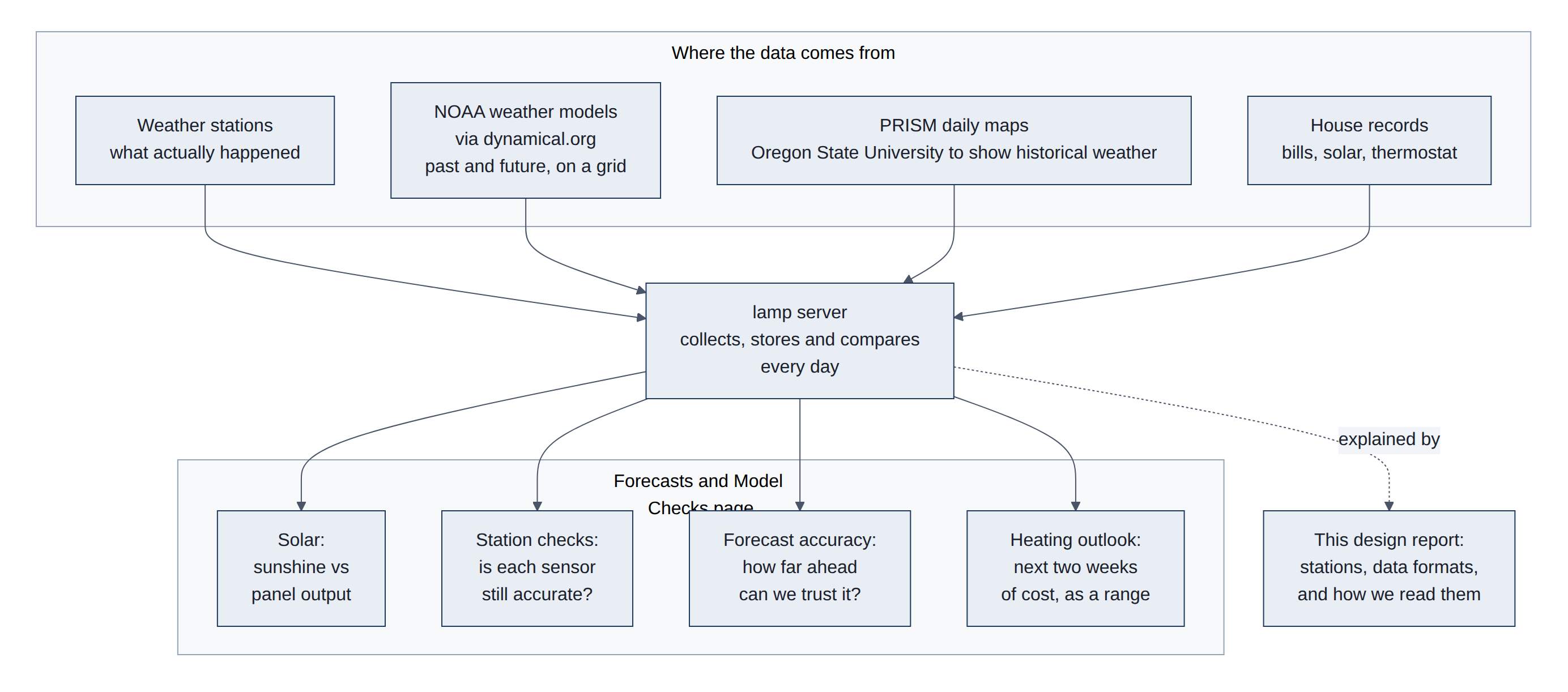
This report has a second goal: the project is a hands-on way to learn cloud-native data formats, a newer way of storing large scientific data on the internet so that a program can read just the small piece it needs. Section 3 explains these formats from the ground up, and sections 4.4 to 7 weigh the one design decision still open.
The results page is built by fc page (forecasting/forecasting/charts/) after each daily update; this page is generated from forecasting/09-direct-access-design.md (see the README, the project's read-me file, for the build command). The analyses on the results page map to use cases and phases in 02-use-cases.md and 04-implementation-plan.md (Table 1):
Table 1. Analyses on the Forecasts and Model Checks page.
| Results page section | Question | Data used | Use case, phase |
|---|---|---|---|
| Solar | Did the panels deliver what the sky allowed? | PRISM daily solar, HRRR sunlight, house pyranometer, SolarEdge production, PVGIS monthly model | U1, Phase 2 |
| Station checks | Has a station drifted? | Station hourly temperature minus the HRRR analysis; daily highs and lows minus PRISM | U2, Phase 2 |
| Forecasts and accuracy | How far ahead is each model useful? | HRRR 48 h and GFS 16-day forecasts, scored against ZASTMET, KPWM and PRISM by lead time | U3, Phase 3 |
| Solar forecast | How much will the panels make in the next days, and how good were past forecasts by lead time? | HRRR and GFS sunlight forecasts, PVGIS model, SolarEdge production | U6 |
| Heating outlook | Next two weeks of heating degree days and cost, with a range | GEFS 31-member ensemble, calibrated on six past heating seasons; gas bills; electric meter | U4, Phase 4 |
| Gas bills forecast ahead | How close would a forecast made 0 to 35 days ahead have come to each gas bill? | GEFS runs replayed for every bill since 2021; gas usage model | U4 |
| Electricity | Household use and net grid use for the next two weeks, and how good past forecasts were | Utility meter and SolarEdge consumption; GEFS temperature; GFS solar forecast | Option 3 |
Every score is reported next to persistence and climatology baselines (bias, mean absolute error (MAE) and, for ensembles, coverage of the range from the 10th to the 90th percentile, p10 to p90), as required by 02-use-cases.md. Section 4.3 explains how each forecast is checked, and section 5.3 gives the results.
1.2 The open design question
dynamical.org, the non-profit that republishes NOAA's model data, offers a small helper library (the "wrapper") that finds and opens its datasets in one call. The project could instead read the storage directly with its own code. Both give identical numbers; they differ in effort, in what the project learns, and in who has to keep the code working when dynamical.org changes something. This is decision D7 (Phase 1M). The owner decided to keep the wrapper until further notice; sections 4.4, 4.5 and 6 lay out the facts so the decision can be revisited.
The wrapper is dynamical-catalog 1.0.1. A direct client would replace it with catalog_direct.py (Appendix A), selected by FC_CATALOG_CLIENT. Migration steps M1 to M7 of the plan are in 07-client-migration.md.
1.3 Structure of this report
Section 2 describes the data: the weather stations and the weather models. Section 3 explains the data formats, first how cloud-native formats differ from traditional ones, then each format in turn. Section 4 describes the methods: the data pipeline, how stations are checked, how each forecast is checked against what happened, and the two ways of reading dynamical.org. Section 5 gives the results: what the station checks found, how cloud-native access compares with the traditional route, and how good each forecast has been. Section 6 weighs the direct-access option, and section 7 states the recommendation.
2. Data
2.1 Weather stations
A weather station is a set of sensors on a pole: a thermometer and humidity sensor inside a vented shield that keeps direct sun off them, a wind cup and vane, a rain gauge, and sometimes a sunlight sensor. Stations differ a lot in quality. An official airport station is professionally maintained and has a fan that pulls air past the thermometer, so sunshine cannot warm it. A consumer station costs a few hundred dollars and relies on still air moving through its shield on its own, so on sunny, calm days it can read a degree or two warm. Any sensor can also drift: its readings slowly shift over months as parts age or the shield gets dirty.
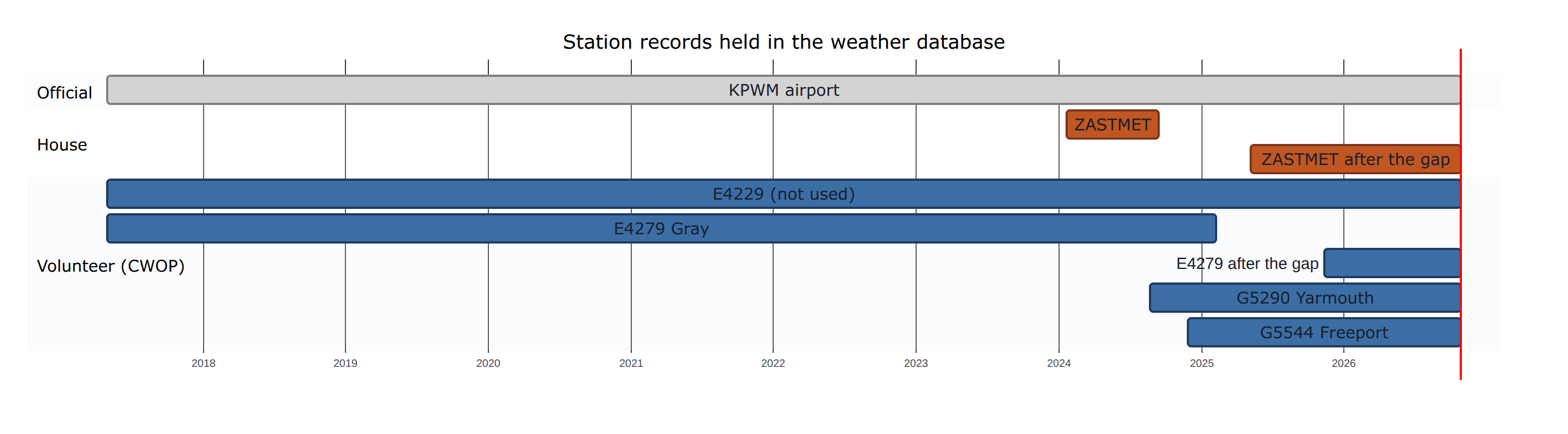
The project collects six stations within about 22 km of the house and analyses five of them. Two, the airport (KPWM) and the house station (ZASTMET), are the "truth" that forecasts are scored against. E4229, a volunteer station of the Citizen Weather Observer Program (CWOP), is still collected but has been left out of every analysis since 2026-10-27, because its readings are faulty (section 5.1.3). The other three are volunteer stations used for comparison and quality checks (Table 2).
Table 2. The weather stations.
| Station | Where | Kind of station | Height above sea level | Readings per day (last 90 days) | Our record |
|---|---|---|---|---|---|
| KPWM | Portland International Jetport, 18 km south | Official airport station (Automated Surface Observing System, ASOS) | 19 m | about 28 | since May 2017 |
| ZASTMET | The house, Cumberland Center | Consumer station, Ambient Weather WS-2902 | 56 m | about 260 (one every 5 minutes) | since Jan 2024, gap Sep 2024 to May 2025 |
| E4229 (not used) | Listed as Cumberland, 22 km northeast | Volunteer (CWOP) | 64 m | about 90 (every 15 minutes) | since May 2017; excluded from analyses since Oct 2026 |
| E4279 | Gray, 17 km northwest | Volunteer (CWOP), Davis Vantage Pro2 | 96 m | about 94 | since May 2017, gap Feb to Nov 2025 |
| G5290 | Yarmouth, 6 km east | Volunteer (CWOP) | 30 m | about 266 | since Aug 2024 |
| G5544 | Freeport, 11 km northeast | Volunteer (CWOP) | 55 m | about 246 | since Nov 2024 |
Three older stations (E1248, G5907 and BARDHAM) went offline and are no longer collected (Figure 2).
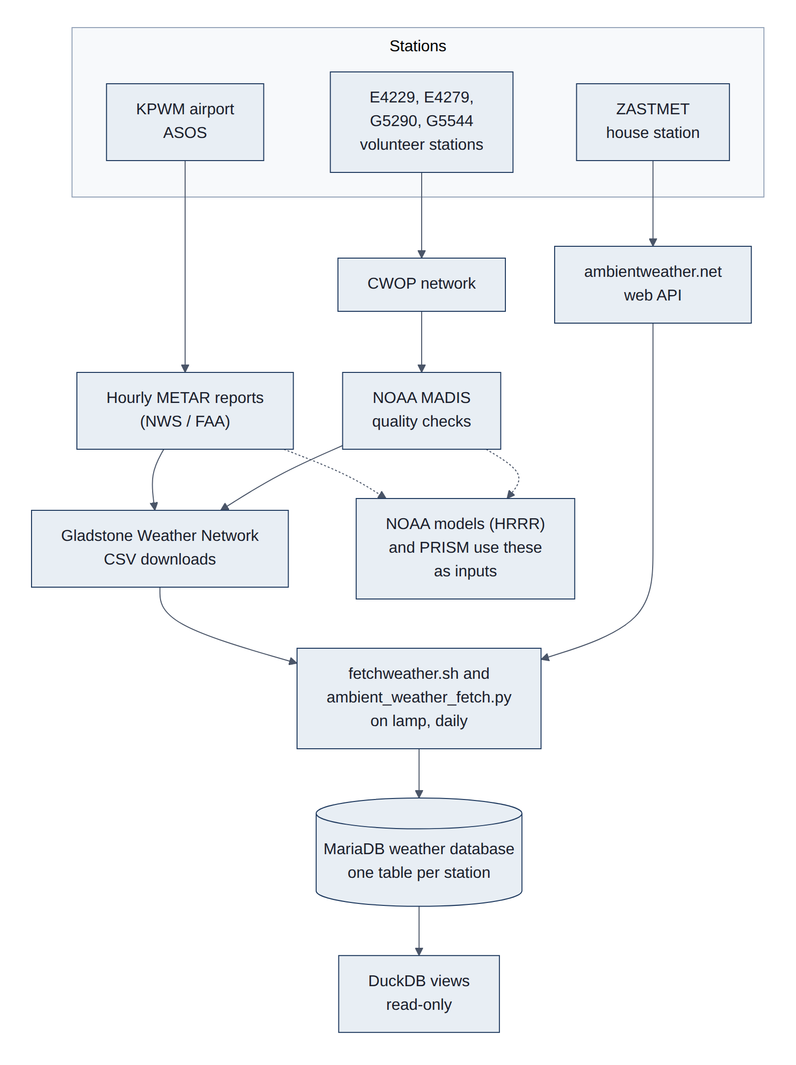
How station data reaches us. Station data arrives the traditional way: as small text files and web responses that a script downloads every day and stores row by row in the project's database (MariaDB). The volunteer stations send their readings to the Citizen Weather Observer Program (CWOP). NOAA's Meteorological Assimilation Data Ingest System (MADIS) service checks those readings for obvious errors, and the Gladstone Weather Network publishes them with quality statistics; fetchweather.sh downloads them from there. The airport's hourly reports (called Meteorological Aerodrome Reports, or METARs) come the same way. The house station posts to ambientweather.net, whose web Application Programming Interface (API) the project reads directly. The house station is not part of CWOP, so NOAA's models never see it, which makes it the cleanest independent test of those models (Figure 3).
2.2 Weather models
A weather model is a computer program that splits the atmosphere into a 3-D grid of boxes and steps the physics of air, water and sunlight forward in time, a few minutes per step. It starts from the best estimate of the weather right now, built from millions of observations (stations, balloons, aircraft, satellites, radar). NOAA runs several models on supercomputers at its National Centers for Environmental Prediction (NCEP) and publishes the results free of charge. dynamical.org, a non-profit, reformats them into cloud-native stores (section 3), which is how this project reads them.
The project uses three NOAA models and one observation-based map product (Table 3):
Table 3. Weather models and map products used.
| Name | Full name | Who | Grid | How often | How far ahead | Used here for |
|---|---|---|---|---|---|---|
| HRRR | High-Resolution Rapid Refresh | NOAA | 3 km squares, continental US | every hour | 18 h (48 h four times a day) | Best estimate of each past hour; next two days |
| GFS | Global Forecast System | NOAA | about 25 km, whole globe | four times a day | 16 days | Forecasts for the next two weeks |
| GEFS | Global Ensemble Forecast System | NOAA | about 25 km to day 10, then about 50 km, whole globe | once a day (the run at 00:00 Coordinated Universal Time, or UTC, as stored here) | 35 days | Ranges for the heating outlook |
| PRISM | Parameter-elevation Regressions on Independent Slopes Model | Oregon State University | 800 m and 4 km, continental US | daily | (not a forecast) | Independent daily truth and 30-year normals |
2.2.1 Kinds of model output
Models produce three kinds of output, and the difference matters:
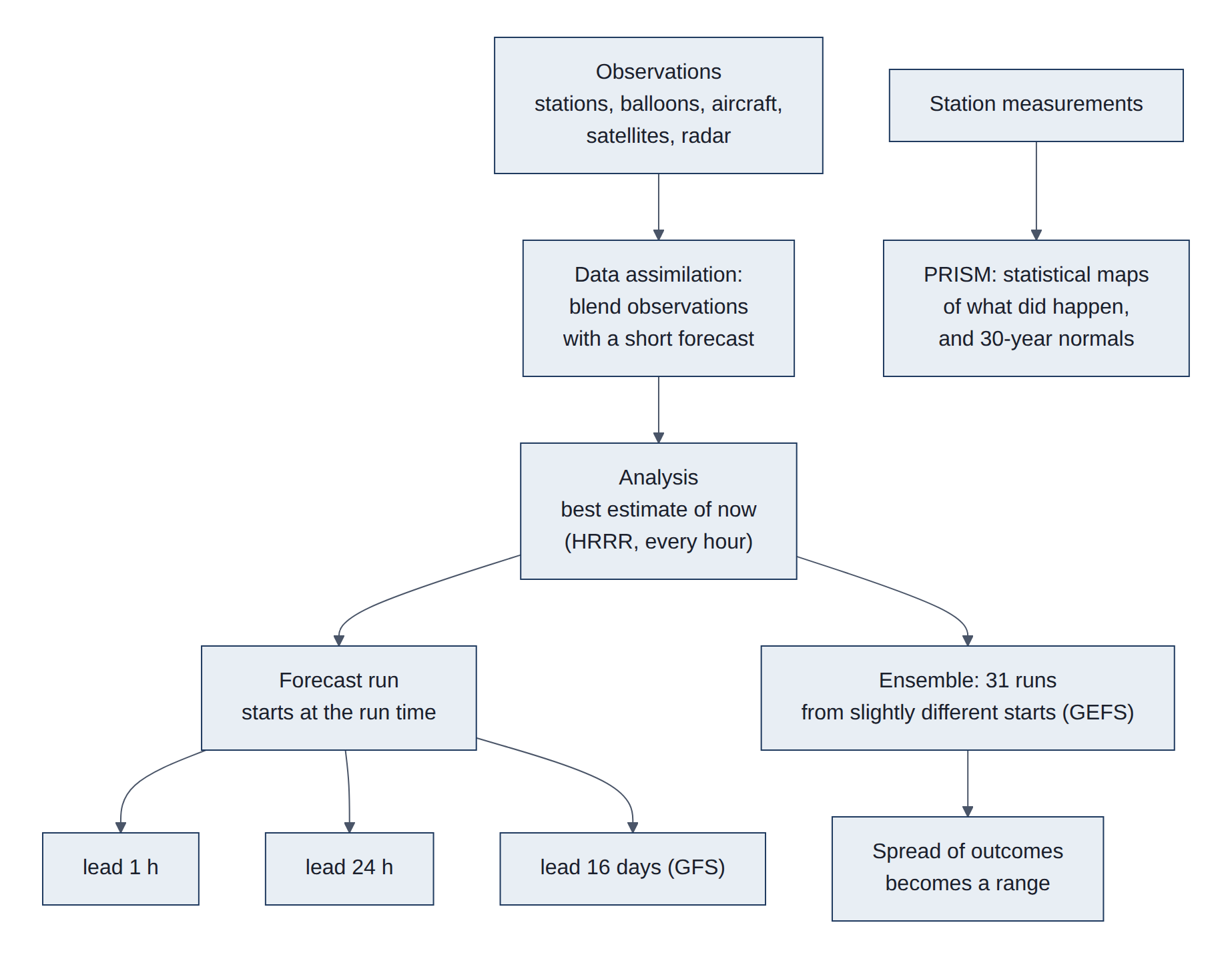
- Analysis. The model's best picture of the weather at a moment that has already happened, made by blending a short forecast with the observations that arrived since. It is not a measurement, but it covers every grid square, including places with no station. HRRR's hourly analyses since 2014 form an hour-by-hour weather history of the whole country.
- Forecast. A run starts at a fixed time (the run time or initialization time, for example "12 UTC on 27 October") and steps forward. Each output is labelled by its lead time, how far ahead of the run time it is ("24 hours ahead"), and its valid time, the moment it describes (run time plus lead time). Forecasts get less accurate as lead time grows; measuring how fast is the job of the forecast accuracy charts.
- Ensemble forecast. One forecast gives one answer, but small errors in the starting picture grow until, after a week or so, they dominate. An ensemble runs the model many times (GEFS: 31 members) from slightly different starting points. Where the members agree, confidence is high; where they spread apart, the future is genuinely uncertain. The heating outlook turns that spread into a range: "8 in 10 chances the cost lands between $51 and $64."
PRISM is different from all three: it is not a physics model and makes no forecasts. It is a statistical method that spreads station measurements across the map, using how temperature and rain change with elevation, slope and distance from the coast. Its output is a daily map of what did happen, plus normals: the average day for each date over 1991-2020, which serve as the "climatology" baseline. PRISM revises each day's map several times over six months as late station reports arrive (Figure 4).
2.2.2 What each output contains
Every model output is a set of variables (temperature, humidity, wind, sunlight, rain and many more), each stored as a grid of numbers. A few details matter for using them correctly:
- Height. Temperature is reported at 2 m above the ground, the height of a station thermometer, and wind at 10 m.
- Instant or total. Temperature is an instant value at the valid time. Rain and sunlight are amounts over a period (an hour, or since the run started); dynamical.org converts them to rates so every hour can be read on its own.
- Map projection. The Earth is round and grids are flat. HRRR uses a Lambert conformal projection, a cone-shaped flattening suited to mid-latitudes, with squares measured in metres. GFS and GEFS use a plain latitude and longitude grid. The project converts the house's latitude and longitude to the right square in each.
- One square, not one spot. A model value describes the average of a whole grid square: 3 km by 3 km for HRRR, roughly 20 km by 28 km for GFS here. A backyard thermometer can differ from it for real reasons, such as a hill, a lake or a parking lot.
Dimensions and the stores the project reads (dynamical.org dataset IDs) (Table 4):
Table 4. dynamical.org datasets read, with dimensions, steps and variables.
| Dataset ID | Model and type | Dimensions | Steps | Variables used here |
|---|---|---|---|---|
noaa-hrrr-analysis | HRRR analysis | time, y, x (Lambert conformal, metres) | hourly since 2014-10 | temperature_2m, dew_point_temperature_2m, relative_humidity_2m, wind_u_10m, wind_v_10m, downward_short_wave_radiation_flux_surface (sunlight), visible_beam_downward_solar_flux_surface, precipitation_surface |
noaa-hrrr-forecast-48-hour | HRRR forecast | init_time, lead_time, y, x | runs every 6 h, hourly leads to 48 h | temperature_2m and the above |
noaa-gfs-forecast | GFS forecast | init_time, lead_time, latitude, longitude (0.25 degree) | 4 runs a day, hourly then 3-hourly leads to 384 h | temperature_2m, maximum_temperature_2m, minimum_temperature_2m |
noaa-gefs-forecast-35-day | GEFS ensemble | init_time, ensemble_member, lead_time, latitude, longitude (0.25 degree; 0.5 degree values interpolated after 240 h) | daily 00 UTC run, 3-hourly leads to 240 h then 6-hourly to 840 h, 31 members | temperature_2m |
Attributes follow the Climate and Forecast (CF) conventions: units, long_name, step_type (instant, avg, accum). The project reduces them to station points (storage layer 2, L2; section 4.1), daily means and heating degree days. Model documentation: HRRR (NOAA Global Systems Laboratory), GFS (NCEP Environmental Modeling Center, EMC), GEFS (NCEP EMC), PRISM (Oregon State University), and the dynamical.org catalog with per-dataset notes. Background on how models work: Numerical weather prediction and Ensemble forecasting. The project's own notes on every model and dataset, including quirks, are in dataset-background.md.
Two other models appear on the results page. PVGIS (Photovoltaic Geographical Information System, from the European Commission's Joint Research Centre) gives expected monthly solar production for the array's tilt and direction (PVGIS). The project's own gas usage model is a straight-line fit of daily gas use against heating degree days, fitted on three years of bills (forecasting/forecasting/energy.py).
3. Background: data formats
3.1 Traditional versus cloud-native formats
A data format is the agreed layout of numbers inside a file, so that the program that wrote them and the program that reads them understand each other. The weather data here comes in six formats (sections 3.2 to 3.8). They fall into two families.
Traditional formats were designed when data lived on a local disk or was copied whole from a server. To use them you download the entire file, then open it. That works for one file, but weather model output is published as one file per model run per forecast hour, each covering the whole country with hundreds of variables. Answering "what was the temperature at my house every hour last year?" means downloading thousands of large files to keep one number from each.
Cloud-native formats are designed for object storage, the internet-scale file storage run by providers such as Amazon's Simple Storage Service (S3), where every file (called an object) has a web address. They rest on one feature of the web: a program can ask a server for just a slice of a file, say bytes 5,000 to 9,000, instead of the whole thing (an HTTP range request; the HyperText Transfer Protocol, HTTP, is how browsers and programs fetch web content). A cloud-native format arranges its contents so that a small, predictable part (the index or metadata) says exactly where every piece of data sits, and the data itself is cut into many separately compressed pieces (chunks). A reader fetches the index, works out which chunks it needs, and fetches only those.
An everyday comparison: a traditional file is like a book without a table of contents that you must photocopy in full to read one page. A cloud-native store is like a library catalog plus numbered shelves: look up the page, walk to the shelf, copy only that page (Figure 5).
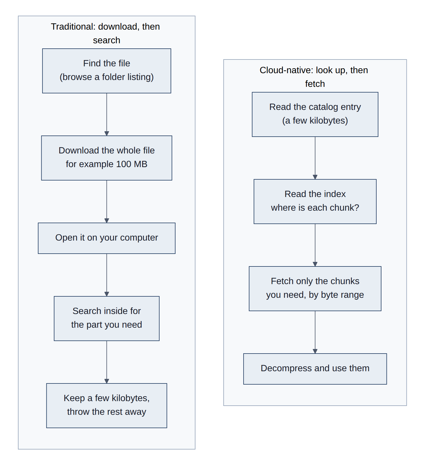
The main ideas, each with its traditional counterpart (Table 5):
Table 5. Main ideas of cloud-native formats and their traditional counterparts.
| Idea | Traditional way | Cloud-native way |
|---|---|---|
| Finding data | Browse folder listings or read documentation | A machine-readable catalog (SpatioTemporal Asset Catalog, STAC) lists every dataset, its variables, dates and address |
| Unit you read | The whole file | A chunk: a small block of the data, fetched by byte range |
| Where the "table of contents" lives | Inside the file, sometimes at the end, spread out, or missing | In a small, separate, predictable place (a metadata file, a manifest, or a fixed spot at the start or end of the file) |
| Layout of the numbers | Arranged the way they were produced: one map per forecast hour, one row per reading | Arranged the way they will be read: long time series for a small area, or one column of a table at a time |
| Compression | The whole file, or not at all | Each chunk on its own, so any chunk can be decompressed alone |
| Updates | Overwrite or add files; a reader can see a half-finished update | New pieces are written first, then one small pointer is switched, so readers see the old version or the new one, never a mix |
| Versions | Usually none: yesterday's file is replaced | Every update is a numbered snapshot, and old ones stay readable |
| Server | Often a special data server that must be running | Plain storage; no server logic, so it scales and rarely breaks |
What it costs. Cloud-native layouts are tuned for an expected kind of question. A store arranged as long time series for small areas is fast for "one place, many hours" and slow for "the whole country, one hour", because that touches many chunks. Each web request also has a fixed delay, so very small chunks waste time; formats group them into larger objects (shards) to compensate. And the tools are younger than the traditional ones.
The table below pairs each traditional format with the cloud-native format that replaces it in this project. Sections 3.3 to 3.8 explain each one in detail (Table 6).
Table 6. Traditional formats and the cloud-native formats that replace them here.
| Job | Traditional format | Cloud-native format used here |
|---|---|---|
| Find datasets | Folder listings, Thematic Real-time Environmental Distributed Data Services (THREDDS) Extensible Markup Language (XML) catalogs | STAC JavaScript Object Notation (JSON) catalog (3.3) |
| Keep versions and make updates safe | Overwritten files, dated folders | Icechunk repository (3.4) |
| Store big grids of numbers | Network Common Data Form (NetCDF) and Hierarchical Data Format 5 (HDF5) files, one per run | Zarr v3 arrays (3.5) |
| Model output as published by NOAA | GRIdded Binary edition 2 (GRIB2) files, one per run and hour | Virtual Zarr references into the same GRIB2 files (3.6) |
| Tables of readings | Comma-separated values (CSV) text files, database rows (MariaDB) | Apache Parquet column files (3.7) |
| Map images of values | Plain GeoTIFF, raw Band Interleaved by Line (BIL) grids | Cloud Optimized GeoTIFF (COG; 3.8) |
Figure 6 contrasts the two ways of storing a large grid.
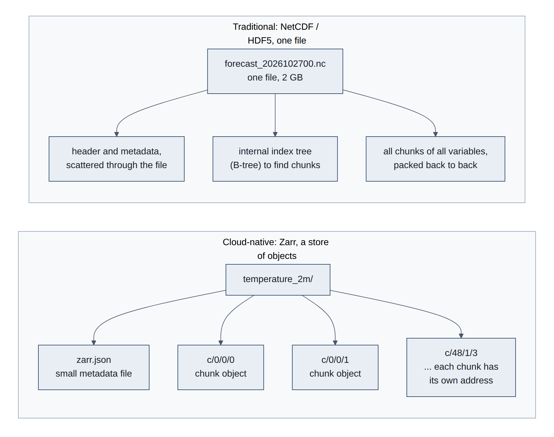
The common thread is metadata first, then byte ranges, with objects that are immutable once written:
- Range reads. Object stores serve
GETwith aRange: bytes=a-bheader (Mozilla Developer Network (MDN): HTTP range requests, Amazon S3 GetObject). Each request costs roughly 20 to 100 milliseconds (ms) of latency against S3, so formats aim for chunks of roughly 1 to 100 megabytes (MB) and issue many requests in parallel. - Locatable metadata. Zarr keeps JSON metadata in a known key; Parquet puts its footer at the end with its length in the last 8 bytes; COG puts all image directories at the start; Icechunk keeps a manifest of every chunk's location. One or two small reads tell the client everything.
- Independent chunks. Each chunk is compressed on its own, so a reader decodes only what it fetched, and many writers can write different chunks at once.
- Immutability and pointer swaps. New data goes to new objects; a commit then updates one small reference with a conditional write. This gives atomic updates and versioning on storage that offers no transactions of its own.
- Contrast with HDF5/NetCDF-4. These are also chunked and compressed, but the chunk index is a B-tree (a balanced tree index) spread through a single file, so a remote reader makes many small dependent reads to walk it, and a single file cannot take concurrent writers. Workarounds exist (HDF5 paged aggregation, Kerchunk and VirtualiZarr references), and dynamical.org uses the reference idea for its virtual GRIB2 stores (3.6).
- Background reading: Zarr: why chunked, cloud-native arrays, Cloud-Native Geospatial Foundation guide to formats, and the Pangeo project on cloud-native analysis of climate data.
3.2 The six formats used here
The project touches six kinds of data containers. Four come from outside: a catalog that says where datasets live, a versioned repository, the grids of numbers inside it, and NOAA's original forecast files. Two are our own: tables of numbers per weather station, and the map images PRISM provides. Each container is built so a program can find and read a small piece without downloading the whole thing; that single idea is what "cloud-native" means here (Figure 7).
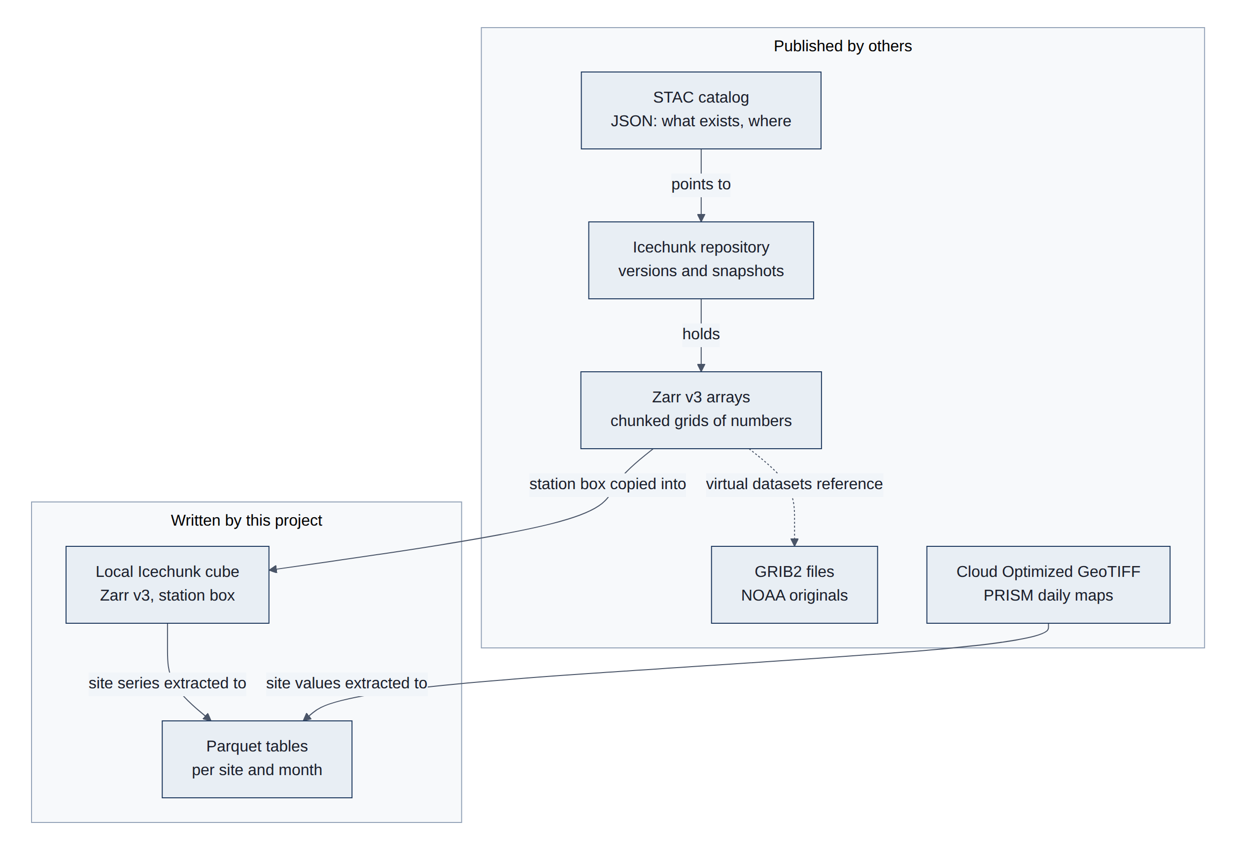
The table names each format, its role here, and the library that reads it (Table 7).
Table 7. The six formats: role, reader library, and whether the project writes them.
| Format | Role in this project | Read with | Written by us |
|---|---|---|---|
| STAC (JSON) | Discover dynamical.org datasets and storage locations | dynamical-catalog (stdlib urllib) | No |
| Icechunk | Versioned, transactional storage for Zarr; remote and our layer 1 (L1) cube | icechunk (Rust core) | Yes (L1) |
| Zarr v3 | Array metadata, chunk grid, codecs | zarr 3.4 via xarray | Yes (L1) |
| GRIB2 | Source of virtual datasets; the traditional format | gribberish codec (virtual), cfgrib/wgrib2 (traditional) | No |
| Parquet | L2 point tables (analysis, PRISM, forecasts) | duckdb, pyarrow | Yes (L2) |
| Cloud Optimized GeoTIFF | PRISM daily grids | rasterio (Geospatial Data Abstraction Library, GDAL) | No |
3.3 STAC catalog
STAC (SpatioTemporal Asset Catalog) is a set of small web documents that describe datasets: their names, dates covered, variables, licence, and the address of the actual data. A program reads the top page, follows the link for the dataset it wants, and gets the address of the repository. It is a table of contents with machine-readable links.
Two terms: JSON (JavaScript Object Notation) is a plain-text way to write structured data, easy for both people and programs to read; a link in STAC is a web address with a label saying what it points to (a child dataset, a licence, the data itself). The traditional counterpart is a folder listing on a web or File Transfer Protocol (FTP) server, or a THREDDS catalog: a person, or a script written for that one site, has to know how the folders and file names are laid out. STAC is a shared standard, so the same code can browse any STAC catalog, from satellite pictures to weather models (Figure 8).
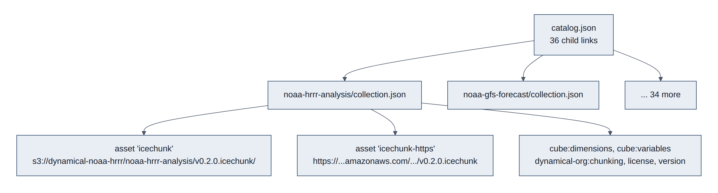
https://stac.dynamical.org/catalog.json is a STAC Catalog whose rel: child links point to one Collection per dataset. A Collection carries (HRRR analysis example) (Table 8):
Table 8. Fields of a dynamical.org STAC Collection (HRRR analysis).
| Field | Content |
|---|---|
assets.icechunk.href | s3://dynamical-noaa-hrrr/noaa-hrrr-analysis/v0.2.0.icechunk/ |
assets.icechunk.xarray:storage_options | {"anon": true, "client_kwargs": {"region_name": "us-west-2"}} |
assets.icechunk-https.href | https://dynamical-noaa-hrrr.s3.us-west-2.amazonaws.com/noaa-hrrr-analysis/v0.2.0.icechunk |
assets.*.icechunk:virtual_chunk_containers | Only on virtual datasets (3.6) |
cube:dimensions, cube:variables | Datacube extension: extents, variables, units |
dynamical-org:chunking | Chunk and shard shapes and byte sizes (3.5) |
version, attribution, license | 0.2.0, attribution text, CC-BY-4.0 |
How it is read: two small HTTPS (secure HTTP) GET requests (catalog, then one Collection), parse JSON, pick the asset by key. The dataset version is in the store path (v0.2.0.icechunk), so a new major version is a new store and the catalog is the only stable way to find it.
Structure in detail. STAC defines three JSON object types (STAC specification):
- Catalog:
id,descriptionandlinks. It only groups other objects. - Collection: a Catalog plus
extent(bounding box and time interval),license,providers,summariesand optional collection-levelassets. - Item: a GeoJSON Feature for one scene or time step, with
geometry,properties.datetimeandassets.
Links carry a rel (self, root, parent, child, item, license). Extensions add fields and are declared by schema Uniform Resource Locator (URL, a web address) in stac_extensions. dynamical.org publishes Collections with collection-level assets and no Items, because each dataset is one continuous array store rather than many files; a satellite-imagery catalog would instead hold one Item per image.
Traditional counterpart. THREDDS catalogs (XML generated by a running server, usually paired with Open-source Project for a Network Data Access Protocol (OPeNDAP) subsetting), International Organization for Standardization (ISO) 19115 metadata records, and directory listings parsed by scripts. Further reading: STAC Index (public catalogs), pystac (Python library), STAC Browser.
3.4 Icechunk repository
Icechunk gives a folder of data files the behavior of a database: changes are saved all at once or not at all, every save gets an ID, and any earlier save can be reopened. dynamical.org saves a new version roughly every hour as model runs arrive. Our own grid cube on lamp is an Icechunk repository too, so the same version history applies to our copy.
Some terms: a commit is one saved change; a snapshot is the complete state of the data after a commit, with its own ID; a branch is a named pointer to the latest snapshot (usually main); a tag is a permanent name for one snapshot. The traditional counterpart is a folder of files that gets overwritten: if the power fails halfway, or someone reads while files are being replaced, they get a mix of old and new, and yesterday's version is gone. Icechunk borrows its ideas from Git, the version-control system programmers use for code, and from table formats such as Apache Iceberg that bring database-style transactions to object storage (hence the name) (Figure 9).
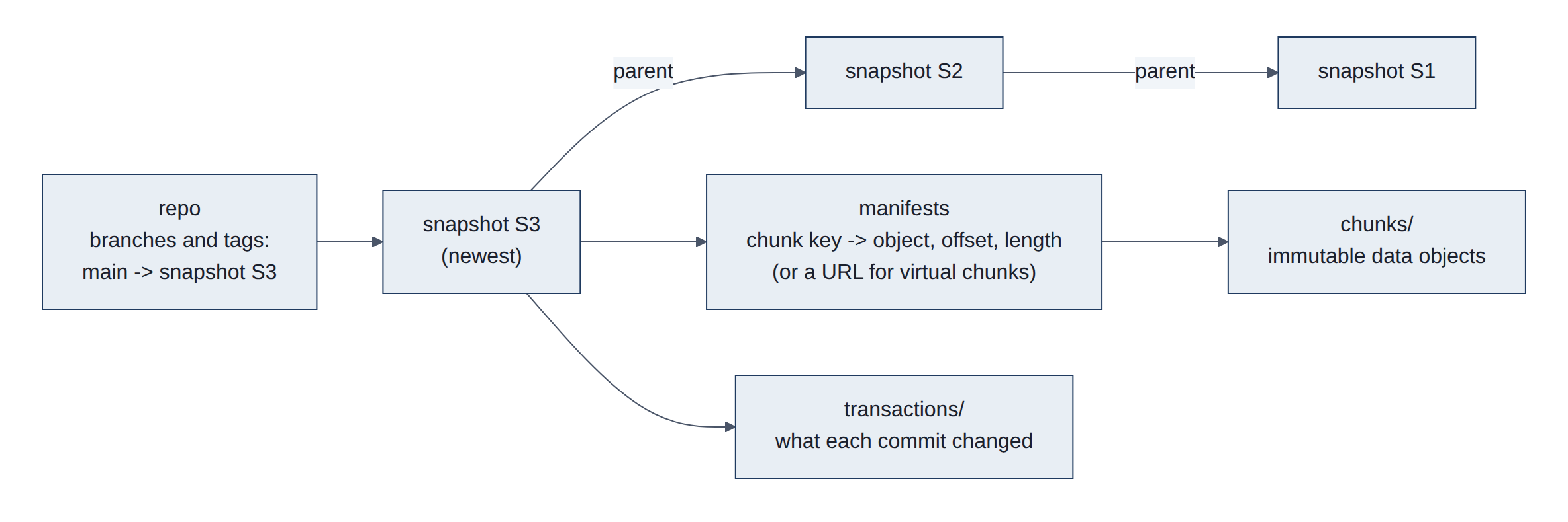
Icechunk (format v2, library 2.3.0) is a transactional storage engine for Zarr on object storage or a local filesystem:
- Objects:
chunks/(immutable data),manifests/(maps from Zarr chunk keys to chunk objects with offset and length, or to external URLs for virtual chunks),snapshots/(a consistent tree: array metadata, attributes, manifest list, parent snapshot),transactions/(the change log per commit), and arepoinfo object holding branch and tag pointers. - Write: a writable session buffers changes;
commit()writes new chunks, manifests and a snapshot, then moves the branch pointer with a conditional write. A concurrent writer loses the race cleanly and must rebase or retry. Nothing is visible until the pointer moves. - Read:
readonly_session("main")orreadonly_session(snapshot_id=...)gives a frozen view; every read in that session sees the same snapshot even if new commits land meanwhile. - Measured, our L1 cube on lamp (
data/cube/hrrr-analysis.icechunk):chunks/564 objects, 225 MB;manifests/578, 0.4 MB;snapshots/50;transactions/50. The remote HRRR analysis repo movesmainabout hourly.
How it is read: open the storage (S3 anonymous, HTTPS or local path), Repository.open, open a session, hand session.store to Zarr. Branch-and-merge for our backfill uses create_branch, commits on the branch, then reset_branch("main", snap, from_snapshot_id=tip) as a compare-and-swap fast-forward.
Structure in detail (Icechunk specification):
- Object IDs are random 12-byte values written in Crockford base32, the 20-character IDs such as
YDHVPTJF7A8TB2D6008Gin our run logs. - A snapshot lists every node (group or array) with its Zarr metadata and, for arrays, the manifests that hold its chunk references, with the chunk-coordinate range each manifest covers. A read loads only the manifests that overlap its selection.
- Manifests can be split by array and coordinate range, so a large array does not need one huge manifest. Very small chunks can be stored inline in the manifest instead of as objects.
- Conflicts: a commit fails if the branch moved since the session started;
rebasewith a conflict solver replays the changes onto the new tip when they touch different chunks. - Maintenance: storage only grows until
expire_snapshotsandgarbage_collectremove objects no longer reachable from a kept snapshot. Our L1 cube keeps everything for now (about 225 MB).
Traditional counterpart. NetCDF files rewritten in place, or versioned folders (v1/, v2/); databases give transactions but not for multi-gigabyte arrays in object storage. The tabular cousins are Apache Iceberg and Delta Lake. For the version-control analogy, see Git internals: objects.
3.5 Zarr v3 arrays, chunks and shards
Inside the repository, each weather variable is a grid of numbers with three directions: time, north-south and east-west. For HRRR temperature that is 105,810 hours by 1,059 by 1,799 cells. The grid is cut into tiles of 90 days by 135 km by 135 km, and groups of 120 tiles are packed into one stored object with a small index at the end. To read one place for one year, a program reads each object's index, then just the few tiles it needs. Numbers are rounded slightly (to about 0.1 degrees Celsius (degC) for temperature) and compressed.
Some terms: an array is a grid of numbers with several directions, called dimensions (here time, north-south and east-west); a chunk is one block of the grid, stored and compressed on its own; a shard is a bundle of chunks stored as one object to save web requests; a codec is one step that encodes or compresses the bytes on the way in and reverses it on the way out; metadata is the description of the data (its shape, type, units and chunk layout) rather than the data itself.
The traditional counterparts are NetCDF (Network Common Data Form) and HDF5 (Hierarchical Data Format version 5), the standard scientific formats for decades. They also cut data into chunks, but keep everything in one large file with its index spread inside it. That suits a local disk but needs many back-and-forth requests over the internet, and only one program can safely write the file at a time. Zarr instead stores each chunk (or shard) as its own object with its own address, plus one small metadata file.
The shape of the chunks decides which questions are fast. dynamical.org makes each chunk a long time series for a small area, because most users ask about places over time (Figure 10):
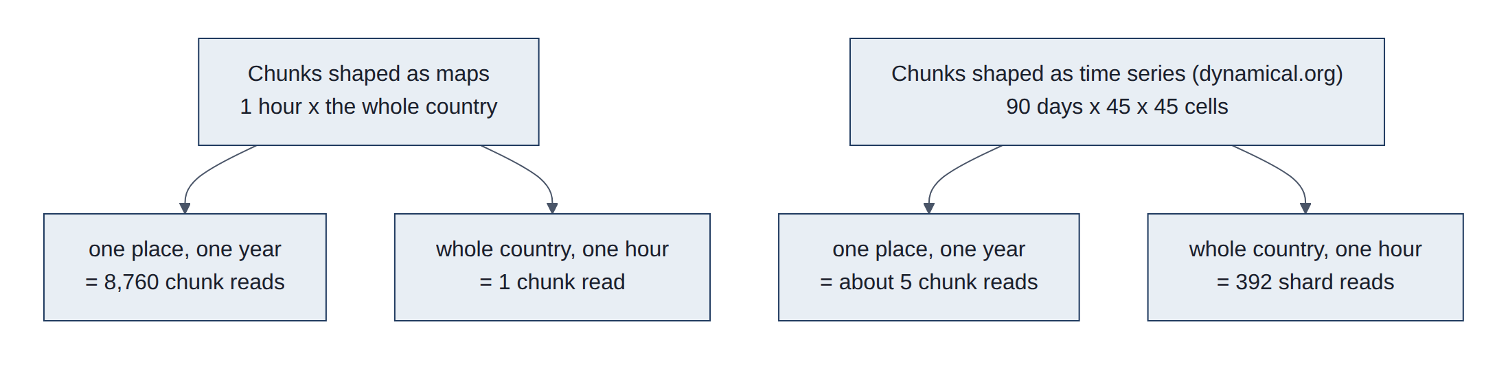
Figure 11 shows how the HRRR temperature array is cut into shards and chunks.
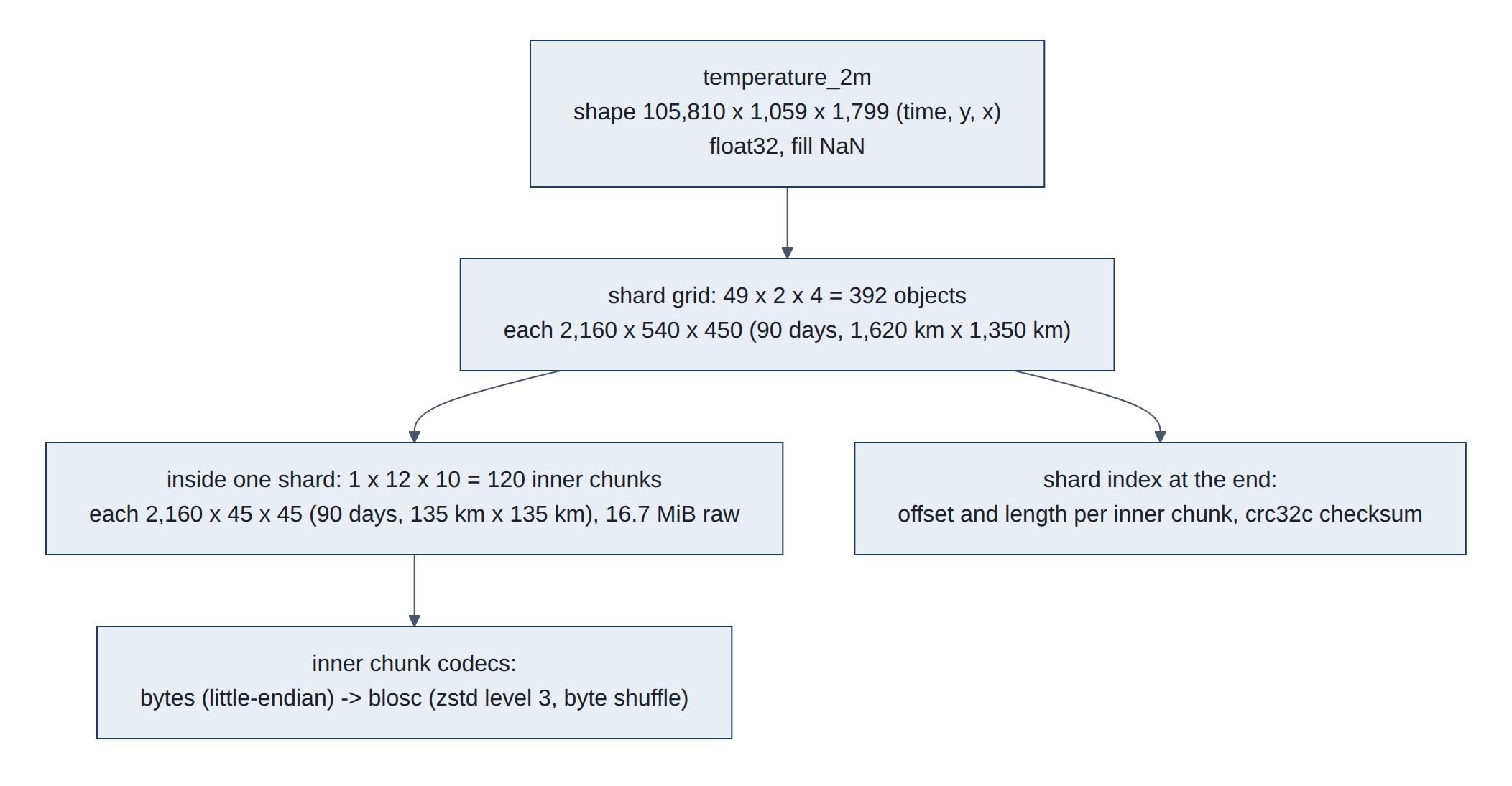
A Zarr v3 array is metadata (zarr.json) plus chunk objects. Read from the live store, the temperature_2m metadata is (Listing 1):
Listing 1. Metadata of the HRRR temperature_2m array (zarr.json), read from the live store.
{
  "shape": [105810, 1059, 1799], "data_type": "float32", "fill_value": "NaN",
  "dimension_names": ["time", "y", "x"],
  "chunk_grid": {"name": "regular", "configuration": {"chunk_shape": [2160, 540, 450]}},
  "codecs": [{"name": "sharding_indexed", "configuration": {
      "chunk_shape": [2160, 45, 45],
      "codecs": [{"name": "bytes", "configuration": {"endian": "little"}},
                 {"name": "blosc", "configuration": {"cname": "zstd", "clevel": 3,
                                                      "shuffle": "shuffle", "typesize": 4}}],
      "index_codecs": [{"name": "bytes"}, {"name": "crc32c"}],
      "index_location": "end"}}]
}- The chunk grid (2160 x 540 x 450) is the shard: one stored object each.
- The sharding codec splits each shard into inner chunks (2160 x 45 x 45) compressed independently, with an index of (offset, length) pairs at the end, checksummed with crc32c (a 32-bit cyclic redundancy check, Castagnoli variant) (sharding spec).
- Blosc with Zstandard (zstd) and byte shuffle groups the bytes of neighboring float32 (32-bit floating-point) values, which compresses smooth fields well; values were mantissa-rounded (about 7 significant bits, 11 for pressure) before writing, which helps further.
- Coordinates (
time,x,y) are small 1-D arrays (timeis int64, a 64-bit integer, with blosc/zstd); CF-style attributes (units,step_type,comment) and root attributes (dataset_id,license, ...) live in metadata.
Figure 12 traces one such read, step by step.
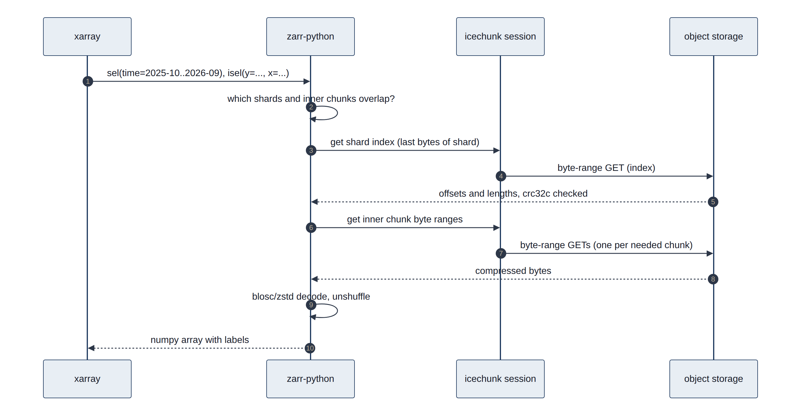
How it is read: xr.open_zarr(session.store, chunks=None, consolidated=False) reads only metadata; selection plus .load() triggers the byte-range reads above. Measured: one variable, one cell, one year is about five inner chunks: 19.3 MB in 1.0 s. Our L1 cube uses the same format with our own chunking (whole station box, 90 days per chunk, no sharding needed at this size) and reached 5.5x compression.
Structure in detail (Zarr v3 core specification):
- Hierarchy: a store holds nodes. The root group's
zarr.jsonis{"zarr_format": 3, "node_type": "group", "attributes": {...}}; each array is a child path (temperature_2m/zarr.json). - Chunk keys: the default encoding names chunk (i, j, k)
c/i/j/k. A chunk that was never written reads asfill_value, so empty regions cost nothing to store. - Codec pipeline: zero or more array-to-array codecs (for example
transpose), exactly one array-to-bytes codec (bytes, orsharding_indexed, which nests its own pipeline per inner chunk), then bytes-to-bytes codecs (blosc,zstd,gzip,crc32c). - v2 versus v3: Zarr v2 used
.zarray,.zattrsand.zgroupfiles; v3 merges them intozarr.jsonand adds sharding anddimension_names. - Conventions: attribute names follow the CF conventions (
units,long_name,standard_name), which is how xarray knows thattimeis a time axis.
Traditional counterpart. NetCDF-4 is a set of conventions on top of an HDF5 file; NetCDF classic has no compression at all. Remote subsetting of either needs a running OPeNDAP or THREDDS server. Further reading: zarr.dev, zarr-python documentation, xarray input and output, NetCDF, HDF5.
3.6 Virtual datasets and GRIB2
NOAA publishes its model output as GRIB2 files: one file per model run and forecast hour, holding many whole-country maps one after another. A "virtual" dataset does not copy those maps; it keeps a list of where each map sits inside NOAA's files and reads it from there when asked. That makes new runs available sooner, but each read pulls a whole map, so it is slow for a single location's history.
GRIB stands for GRIdded Binary. It is the World Meteorological Organization's standard for exchanging model output, and edition 2 has been in use since the early 2000s. To save space it packs numbers tightly: instead of storing each temperature as a full-precision number, it stores small whole numbers plus a recipe (a reference value and scale factors) to turn them back into temperatures. A message is one map of one variable at one height and one time. A virtual dataset holds addresses that point into someone else's files, not copies of the data (Figure 13).
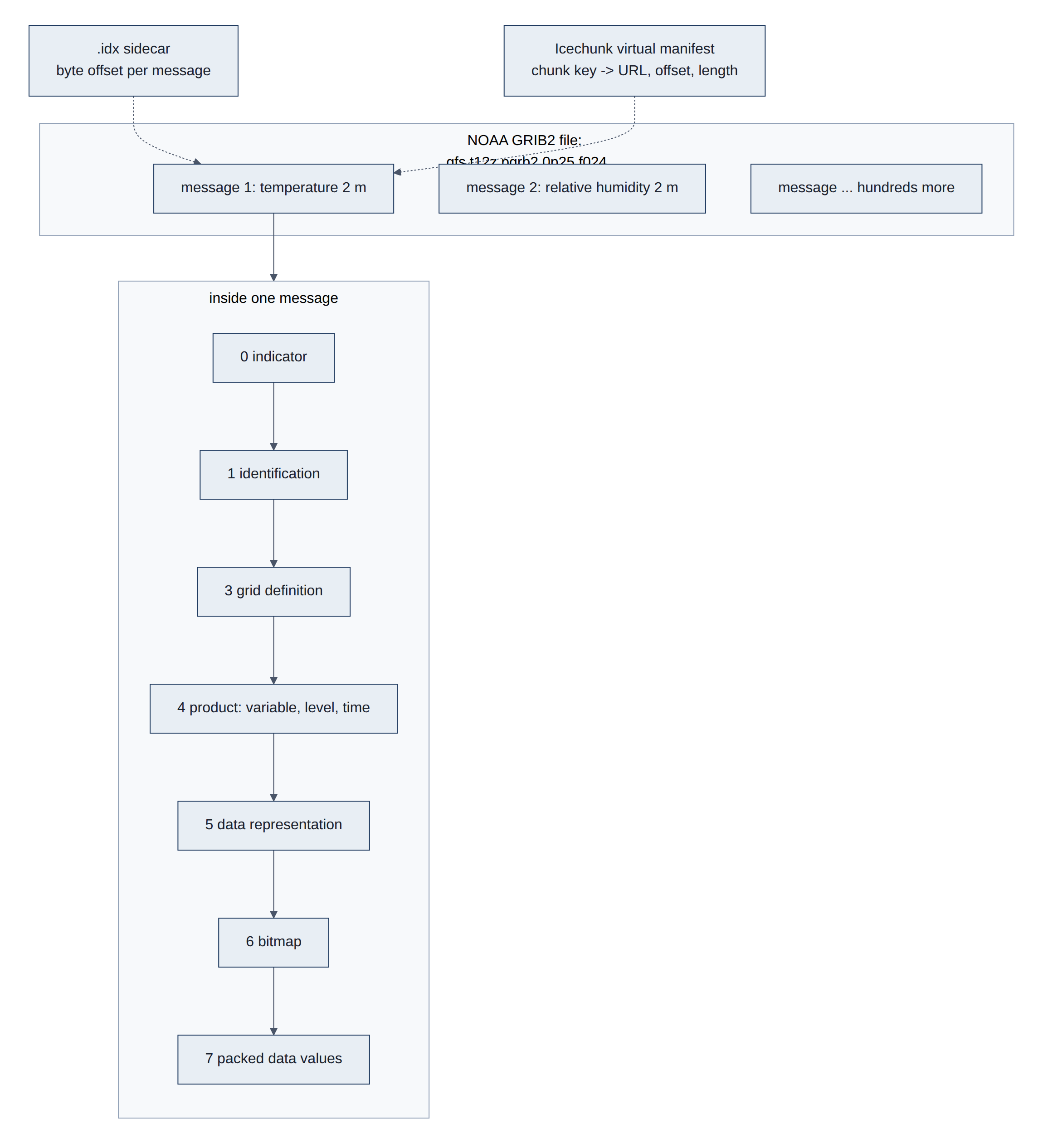
- GRIB2 (World Meteorological Organization (WMO) code form FM 92) is a stream of self-describing messages; each holds one 2-D field with sections for grid, product (variable, level, forecast time) and packed data (simple, complex or JPEG2000 packing). NOAA also publishes
.idxtext sidecars with each message's byte offset, which allow byte-range reads of single messages. - Virtual Icechunk stores keep manifest entries that point to (URL, offset, length) inside the GRIB2 objects (for GFS,
s3://noaa-gfs-bdp-pds/). Chunks are whole fields:1 x 1 x 721 x 1440(one run, one lead, the globe; 7.9 mebibytes (MiB) raw, float64, the 64-bit version). - Reading needs two things the materialized stores do not: authorization of each external container at open time (
authorize_virtual_chunk_accesswith anonymous credentials listed in the Collection), and thegribberishcodec, which decodes a GRIB2 message as a Zarr chunk. - Measured (arrival logger): GFS 12Z appeared in
noaa-gfs-forecast-virtualat 17:17 UTC while the materializednoaa-gfs-forecaststill showed 06Z at 17:26 UTC.
Structure in detail. Each GRIB2 message has numbered sections (NCEP GRIB2 documentation and code tables) (Table 9):
Table 9. Sections of a GRIB2 message.
| Section | Content |
|---|---|
| 0 Indicator | The bytes GRIB, discipline (0 = meteorological), edition 2, total message length |
| 1 Identification | Originating centre (7 = NCEP), reference (run) time, production status |
| 2 Local use | Optional, centre-specific |
| 3 Grid definition | Template 3.0 regular latitude/longitude (GFS), 3.30 Lambert conformal (HRRR) |
| 4 Product definition | Parameter as discipline/category/number (0/0/0 = temperature), level (type 103 = height above ground, 2 m), forecast time; template 4.0 instantaneous, 4.8 statistics over an interval (accumulations, averages), 4.1 and 4.11 ensemble members |
| 5 Data representation | Packing: 5.0 simple, 5.3 complex with spatial differencing, 5.40 JPEG 2000 (Joint Photographic Experts Group 2000 standard) |
| 6 Bitmap | Which grid points are missing |
| 7 Data | The packed values |
| 8 End | The bytes 7777 |
With simple packing a value is Y = (R + X x 2^E) / 10^D, where X is the stored N-bit integer, R a reference value, and E and D binary and decimal scale factors. Sections 2 to 7 may repeat inside one message. A line of a .idx sidecar looks like 1:0:d=2026102612:TMP:2 m above ground:24 hour fcst: (message number, byte offset, run time, variable, level, lead).
Traditional tools: wgrib2, ecCodes and cfgrib. Pitfalls dynamical.org handles for us: accumulations that reset at different intervals, winds relative to the Lambert grid rather than to north, and variables that appear only at some lead times. Further reading: VirtualiZarr and Kerchunk (building virtual references), NOAA HRRR on Amazon Web Services (AWS).
3.7 Parquet tables (our L2)
Parquet is a file format for tables that stores each column separately and compressed, with a summary at the end saying what range of values each column holds. Our tables are split into folders by data source, station, year and month, so a question about one station and one month opens one small file, and a program can skip files whose summaries rule them out without reading them.
Some terms: a row is one record (one reading at one time); a column is one field across all records (every temperature). Traditional tables, a CSV (comma-separated values) text file or a database such as MariaDB, store data row by row, so averaging one column still means reading every field of every row. Parquet stores each column together. It reads only the columns asked for, and similar values side by side compress very well. It also records the smallest and largest value of each column in each block, so a question about "September 2026 only" skips blocks that cannot match.
The catch: a Parquet file is written once and replaced, not edited row by row. That suits history and analysis, while a database suits constant small updates. This is why the station readings stay in MariaDB, and the analysis tables built from them are Parquet (Figure 14).
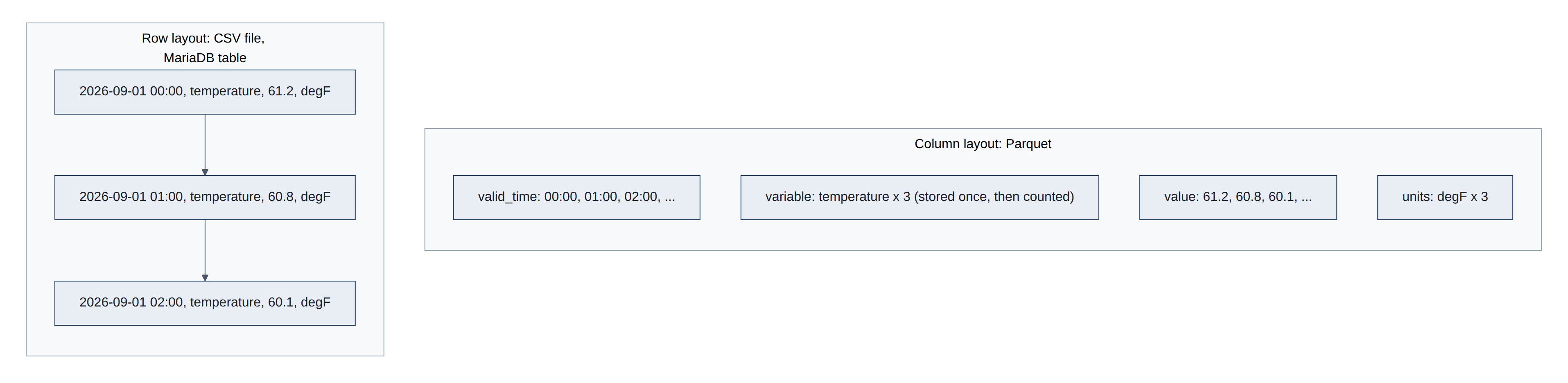
Figure 15 shows the partition folders and the inside of one of these files.
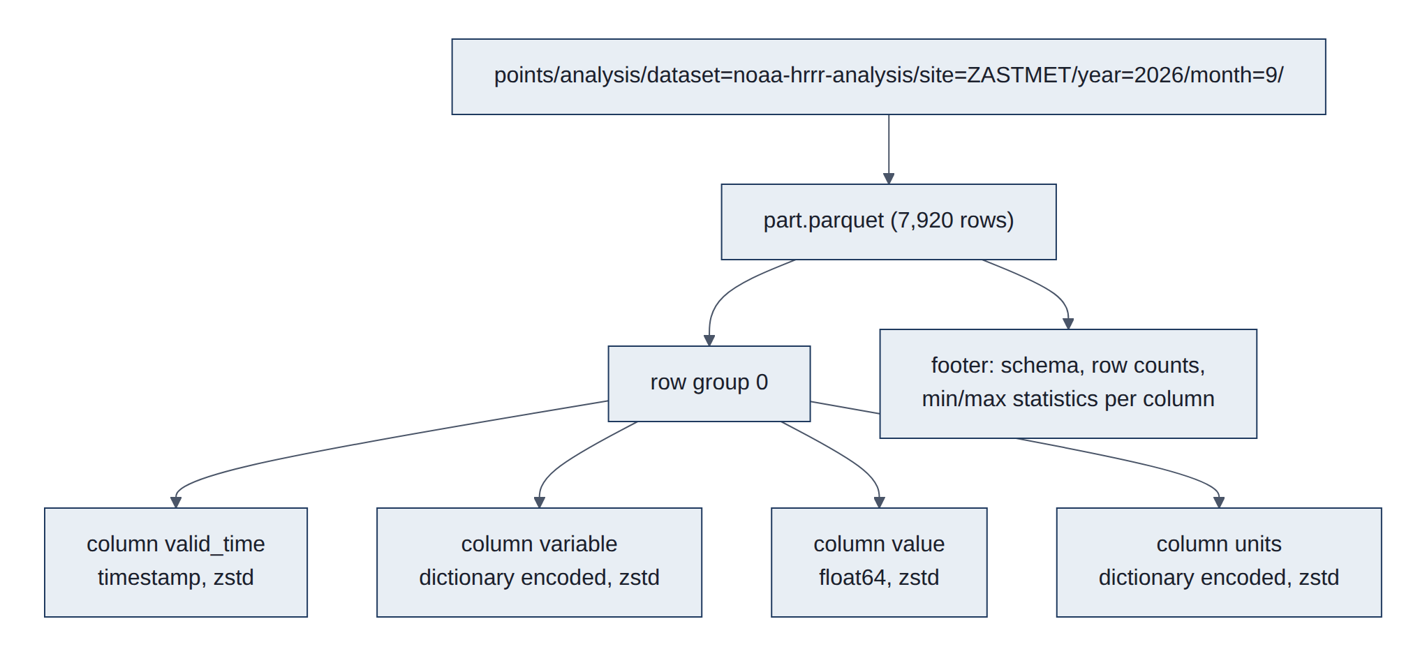
Parquet files start and end with the magic PAR1; data is split into row groups, each holding one column chunk per column, each column chunk made of pages (a dictionary page plus data pages). The footer holds the schema and per-column statistics. Read from our file (site=ZASTMET/year=2026/month=9): 7,920 rows, one row group, written by parquet-cpp-arrow 26.0.0, every column zstd with dictionary encoding; valid_time statistics 2026-09-01T00:00Z to 2026-09-30T23:00Z; compressed column sizes 4.4 kilobytes (KB) (valid_time), 0.4 KB (variable), 19.8 KB (value), 0.3 KB (units).
- Hive partitioning:
key=valuefolder names become columns (dataset,site,year,month) when DuckDB reads withhive_partitioning = true, and filters on them skip whole folders. - Long format (
valid_time, variable, value, units) means a new variable needs no schema change; the dictionary encoding keeps the repeatedvariableandunitsstrings tiny. - Writes are whole-partition: write
part.parquet.tmp, compare bytes with the existing file, thenos.replace(atomic on one filesystem). Identical bytes mean no rewrite, which makes re-runs idempotent.
How it is read: DuckDB reads each footer first, prunes partitions by path and row groups by min/max, then reads only the needed column chunks: read_parquet('<points>/analysis/**/*.parquet', hive_partitioning = true).
Byte layout of a file: PAR1 | row group 1 ... row group n | footer | 4-byte footer length | PAR1. A row group holds one column chunk per column; a column chunk is a sequence of pages (an optional dictionary page, then data pages, each with a small header). The footer is a Thrift-encoded FileMetaData: the schema, key-value metadata (pyarrow stores the Arrow schema there), and for every row group and column the byte offset, sizes, encodings, compression codec and statistics (min, max, null count). A reader fetches the last 8 bytes, then the footer, then only the column chunks it needs.
- Encodings:
PLAIN;RLE_DICTIONARY(a dictionary of distinct values plus run-length and bit-packed indexes, used for ourvariableandunitsstrings);DELTA_BINARY_PACKED(integers and timestamps);BYTE_STREAM_SPLIT(floats). - Missing values and nesting: definition and repetition levels, the scheme from Google's Dremel paper.
- Optional indexes: a page index (min and max per page) and Bloom filters for fast "is this value present?" checks.
- Logical types:
TIMESTAMP(with unit and an "adjusted to UTC" flag),DATE,DECIMAL,STRING.
Traditional counterpart. CSV (Request for Comments (RFC) 4180) is untyped text that must be parsed in full. MariaDB's InnoDB engine stores rows in B-tree pages ordered by primary key, which is ideal for looking up or updating one record and slow for scanning one column of millions. Further reading: Parquet file format, Parquet encodings, DuckDB: reading Parquet, DuckDB: Hive partitioning, Apache Arrow (the in-memory column format behind pyarrow).
3.8 Cloud Optimized GeoTIFF (PRISM)
PRISM publishes each day's map as a GeoTIFF image whose pixels are values (solar energy, temperature, rain) instead of colors. "Cloud optimized" means the image is cut into square tiles with a table of where each tile starts, plus smaller preview copies, so a program can fetch one tile. PRISM wraps the image in a zip file, though, and zip compression hides the tile positions, so we download the whole 2.7 MB file and read our station points from it.
Some terms: a raster is a picture made of a grid of cells (pixels), here each holding a number rather than a colour; GeoTIFF is the long-standing Tagged Image File Format (TIFF) picture format plus tags that say where on Earth each pixel lies; a tile is a square block of pixels; an overview is a smaller, coarser copy of the whole picture for zoomed-out views.
A plain GeoTIFF often stores its pixels in strips (whole rows across the map), may keep its table of contents at the end of the file, and has no overviews, so a program usually downloads the whole file. Older PRISM downloads used the BIL (band interleaved by line) format: raw numbers plus a separate header text file, also downloaded whole. A COG is still a valid GeoTIFF that any older tool can open; it simply orders its contents so that one small read at the start reveals where every tile is (Figure 16).
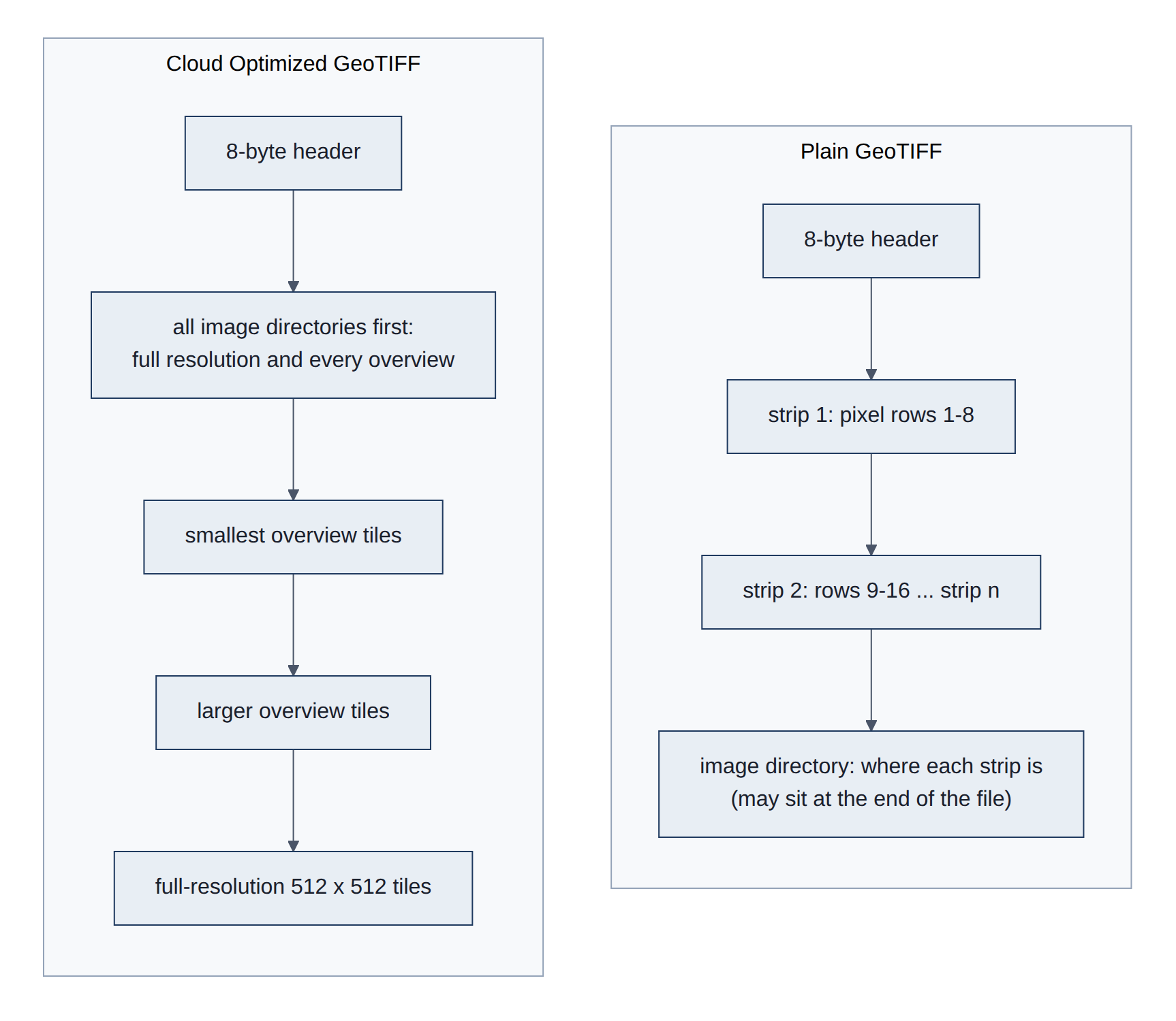
Figure 17 shows what a PRISM daily download contains.
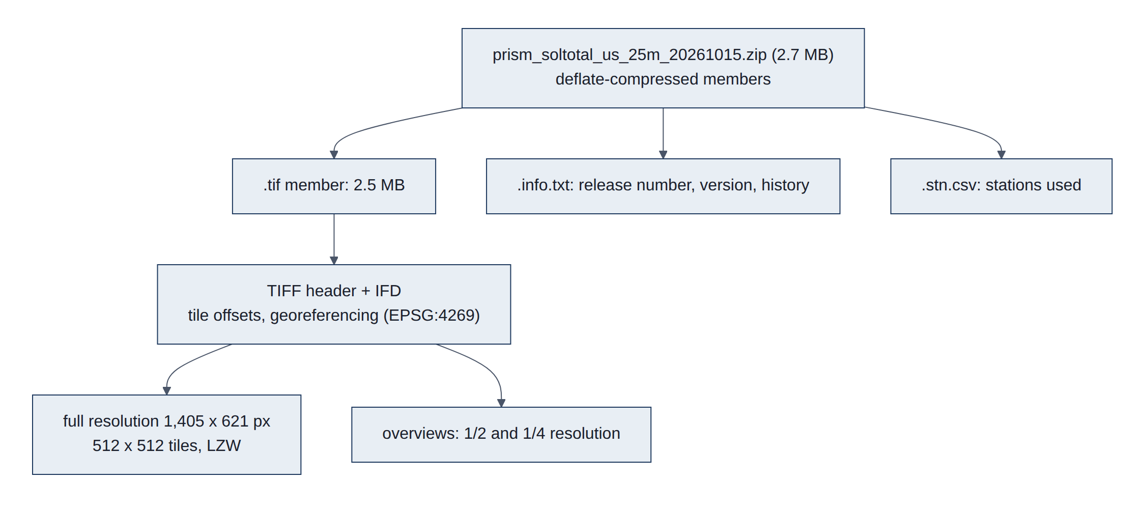
Read from a live grid: 1,405 x 621 pixels (4 km, 2.5 arc-minutes), float32, North American Datum of 1983 (NAD83; code EPSG:4269 in the list kept by the European Petroleum Survey Group, EPSG), LAYOUT=COG, 512 x 512 tiles, Lempel-Ziv-Welch (LZW) compression, overviews at factors 2 and 4, nodata -9999. The zip member is deflate-compressed (2,523,069 bytes to 2,451,079), so the TIFF's byte offsets refer to the inflated stream and HTTP range reads into the zip cannot reach a tile. GDAL's /vsizip/ reads the member in place after download, with no extraction step.
How it is read: rasterio.open("/vsizip/<zip>/<name>.tif").sample([(lon, lat), ...]) reads the Image File Directory (IFD), then only the tiles holding the requested points. The .info.txt member supplies PRISM_DATASET_RELEASE_NUMBER (the revision count) and PRISM_DATASET_VERSION.
Structure in detail. A TIFF starts with an 8-byte header: byte order (II little-endian or MM big-endian), the number 42 (43 for BigTIFF, which uses 64-bit offsets for files over 4 gigabytes (GB)), and the offset of the first IFD (image file directory). Each IFD is a count followed by 12-byte entries (tag, type, count, value or offset) and the offset of the next IFD. Tags that matter here:
ImageWidth,ImageLength,TileWidth,TileLength,TileOffsets,TileByteCounts;Compression(5 = LZW, 8 = Deflate, 50000 = Zstandard),Predictor,SampleFormat(3 = floating point);- georeferencing:
GeoKeyDirectoryTag(the coordinate reference system),ModelPixelScaleTagandModelTiepointTag(pixel to map coordinates), and GDAL'sGDAL_NODATA.
The Open Geospatial Consortium (OGC) COG standard requires tiling and all IFDs at the start. GDAL's COG driver also writes the smallest overview's tiles first and full resolution last, and records the layout in a small "ghost" header area. Further reading: cogeo.org, GDAL COG driver, OGC GeoTIFF standard, rasterio, PRISM data.
4. Methods
4.1 Data pipeline and libraries
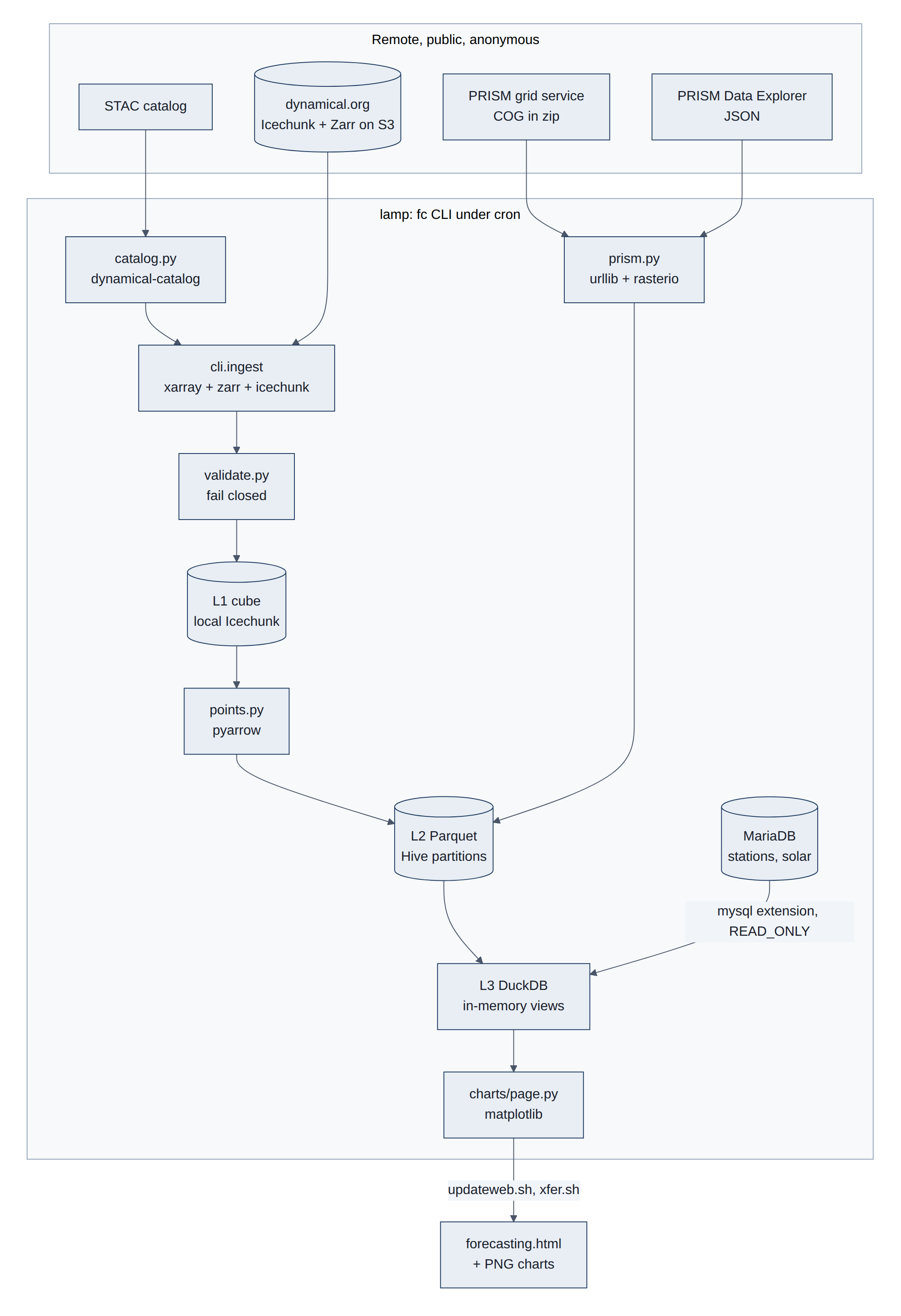
Every day, lamp checks for new data from two outside sources, NOAA model data (through dynamical.org) and PRISM. It keeps a copy of the model grid around the stations, pulls each station's values into small tables, combines them with the house's own weather station and solar records, and draws the charts on the forecasting web page. Each step uses a library designed for one format, so every piece of data stays in the format best suited to how it is used (Figure 18).
The library stack, from our code down to storage (versions on lamp, 2026-10-26) (Figure 19):
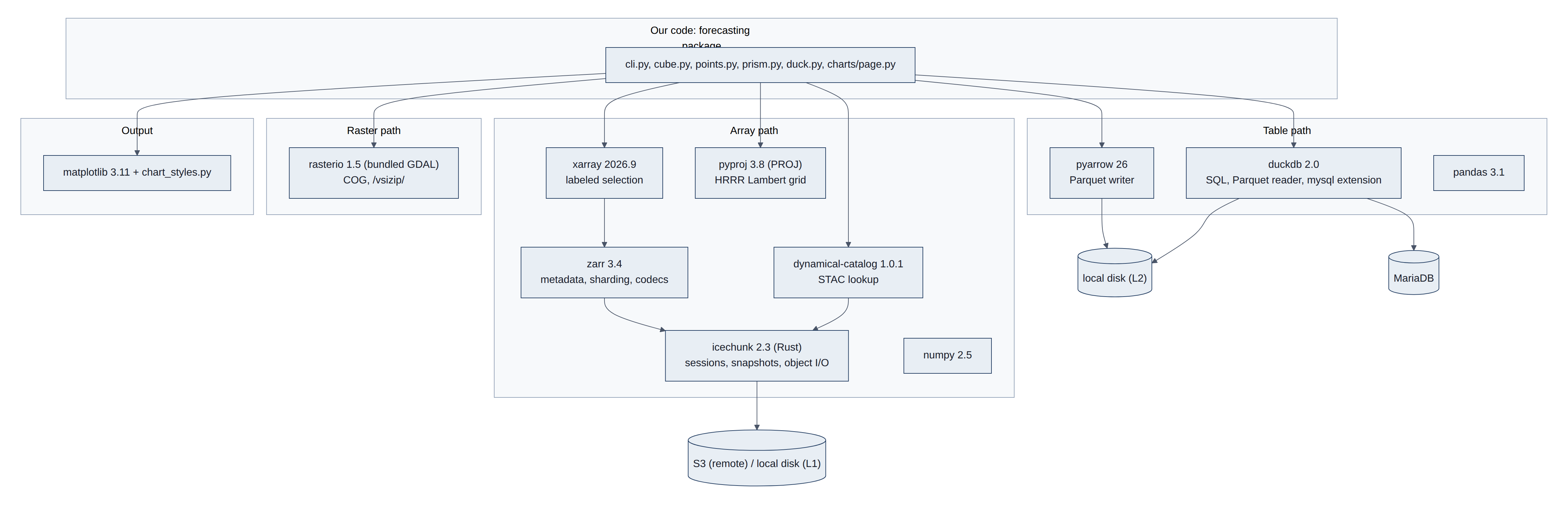
Table 10 lists each library, what it does here, and the format it handles.
Table 10. Libraries and the formats they handle.
| Library | What it does here | Format |
|---|---|---|
dynamical-catalog 1.0.1 | Reads the STAC catalog, builds anonymous storage, opens repositories | STAC, Icechunk |
icechunk 2.3.0 | Sessions and snapshots, object reads and writes, local L1 repos | Icechunk |
zarr 3.4.1 | Array metadata, chunk grid, sharding index, blosc/zstd codecs | Zarr v3 |
xarray 2026.9.0 | Labeled dimensions, selection by time and place, CF attributes | Zarr v3 |
pyproj 3.8.0 | Lat/lon to HRRR Lambert x/y; wind rotation angle | (PROJ library) |
numpy 2.5, pandas 3.1 | In-memory arrays and frames | |
pyarrow 26.0.0 | Writes L2 Parquet (zstd, dictionary encoding, statistics) | Parquet |
duckdb 2.0.0 | Structured Query Language (SQL) views over Parquet; MariaDB attach (mysql extension, READ_ONLY) | Parquet |
rasterio 1.5.2 (GDAL) | PRISM COG sampling inside zips | COG |
gribberish 1.9.0 | GRIB2 codec, installed with the wrapper; used only by virtual datasets | GRIB2 |
matplotlib 3.11 | Charts for forecasting.html | Portable Network Graphics (PNG) |
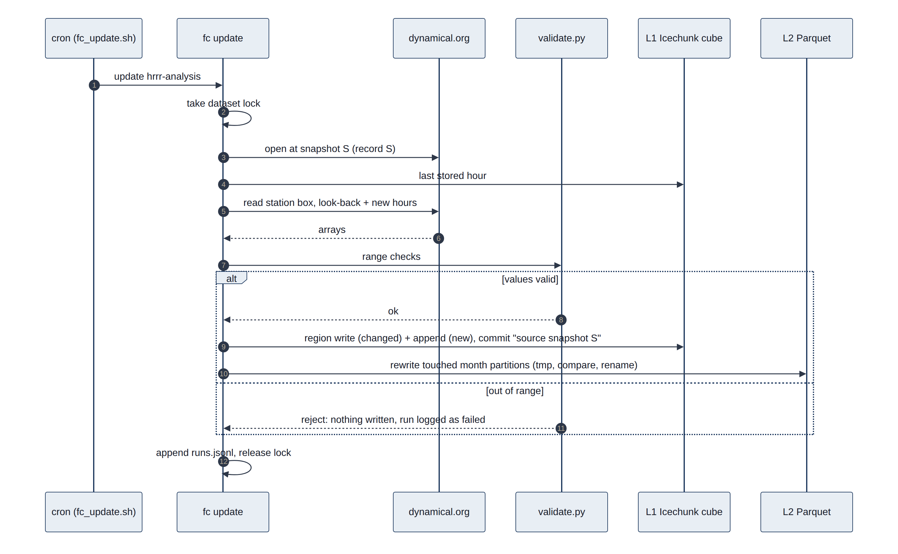
The write path for one update run (L1 then L2) (Figure 20):
4.2 Station quality checks
No station is perfect, so each one is compared with two independent references at the same location:
- The HRRR analysis: NOAA's best estimate of the weather each hour on a grid of 3 km squares, made by blending a weather model with all available observations. Comparing a station with the HRRR square it sits in shows its offset (how much warmer or colder it reads, on average).
- PRISM: daily maps of high and low temperature from Oregon State University, built from thousands of stations and adjusted for terrain.
A steady offset is normal, because a 3 km square is not the same as one spot in one backyard. What matters is a change in the offset, which means something changed at the station.
Offsets against PRISM use days with readings in at least 22 of 24 hours, the PRISM day window (12:00 UTC to 12:00 UTC, labelled by its end date), and station max and min of all readings in that window. The HRRR comparison is hourly: the station's hourly mean minus the HRRR analysis at the station's grid cell (fc_zastmet_vs_hrrr in sql/analysis_wx.sql). Independence matters: HRRR assimilates METAR (so KPWM agrees closely by design) and MADIS mesonet data (probably including the CWOP stations), and PRISM uses KPWM and likely some CWOP stations as inputs (08-phase0-results.md section 7). ZASTMET feeds neither, so it is the only fully independent check.
4.3 Forecast checks
Every forecast on the results page is checked against what actually happened, once that is known. Five analyses do this, one for each thing the house cares about: temperature, solar production, heating degree days, the gas bill and electricity use. They share one method, described first, then each analysis in turn. Table 11 summarises them.
Table 11. The forecast checks: what is forecast, what it is checked against, and the baselines it must beat.
| Analysis | Forecast | Checked against (truth) | Baselines | Scores | Results page |
|---|---|---|---|---|---|
| Temperature | Hourly temperature from HRRR (to 48 hours) and GFS (to 16 days); daily high and low | House station (ZASTMET) and airport (KPWM) at the top of each hour; PRISM daily high and low | Persistence; climatology (hourly 2015-2024, daily 1991-2020 normals) | Bias, MAE and skill by lead time, last 90 days | Figures 1-3 |
| Solar production | Daily kilowatt-hours (kWh) from forecast sunlight (HRRR days 0-1, GFS days 0-15) | SolarEdge daily production | Persistence (last full day's production); normal (1991-2020 sunlight for the date) | Bias, MAE and skill by lead day, last 90 days; known-weather floors | Figures 12-13 |
| Heating degree days | Daily and weekly heating degree days from the GEFS ensemble, with an 80% range | KPWM daily mean temperature | Persistence; normal (PRISM 1991-2020 at the station) | MAE, skill and range coverage by lead day, heating seasons since October 2020 | Figures 4-6 |
| Gas bill | Therms for each billing period, from forecast heating degree days | The gas bill (billed therms) | Normal weather; persistence for the unobserved days | Mean absolute error per bill (%, therms, dollars) by days before the meter read | Figures 7-8 |
| Electricity | Daily household use from GEFS temperature plus the recent level; net grid use with the GFS solar forecast | Daily use from the utility meter and SolarEdge | Persistence; normal; normal plus recent level | Bias, MAE, skill and range coverage by lead day since October 2020; weekly totals; net use over the last 90 days | Figures 15-17 |
4.3.1 How a forecast is scored
Four ideas recur in every check.
- Lead time is how far ahead a forecast was made. A forecast for tomorrow made today has a lead of one day. Forecasts get worse as the lead grows, so every score is broken down by lead.
- Error measures. The bias is the average error with its sign: a positive bias means the forecast ran high. The mean absolute error (MAE) is the average size of the error, ignoring its sign; it is the main score, and smaller is better (0 is perfect).
- Baselines. A forecast is only useful if it beats a simple guess that needs no model. Persistence guesses that the future will be like the latest observation ("tomorrow will be like today"). Climatology, or the normal, guesses the average for that date over 1991-2020. The skill score compares the two: skill = 1 - MAE of the forecast / MAE of the baseline. A skill of 1 is a perfect forecast, 0 is no better than the baseline, and below 0 is worse (Murphy 1993).
- Ranges. An ensemble forecast gives a range, here the band that should contain the actual value 8 times in 10 (from the 10th to the 90th percentile, p10 to p90). Its coverage is how often the actual value really fell inside; the target is 80%.
- Uncertainty. A score is an average over a limited sample, so the dated results reports give a 95% confidence interval (CI) for each one. It comes from a moving-block bootstrap#Block_bootstrap): the scored days are resampled in runs of 7 consecutive days, 2,000 times, and the middle 95% of the recomputed scores forms the interval. Whole weeks are drawn because weather errors persist for several days; gas bills are drawn in runs of 3. A forecast is clearly better than a baseline when the lower end of its skill interval is above zero.
A useful way to read the solar and gas checks is to split the error into two parts. Even with perfect knowledge of the weather, turning weather into kWh or therms is not exact: panels get snow and shade, and a house uses gas for hot water and cooking as well as heat. This is the usage-model error, measured by feeding the observed weather into the same calculation (the known-weather floor, or lead 0). The rest of the error, the gap between a forecast's score and the floor, comes from forecasting the weather (Figure 21).
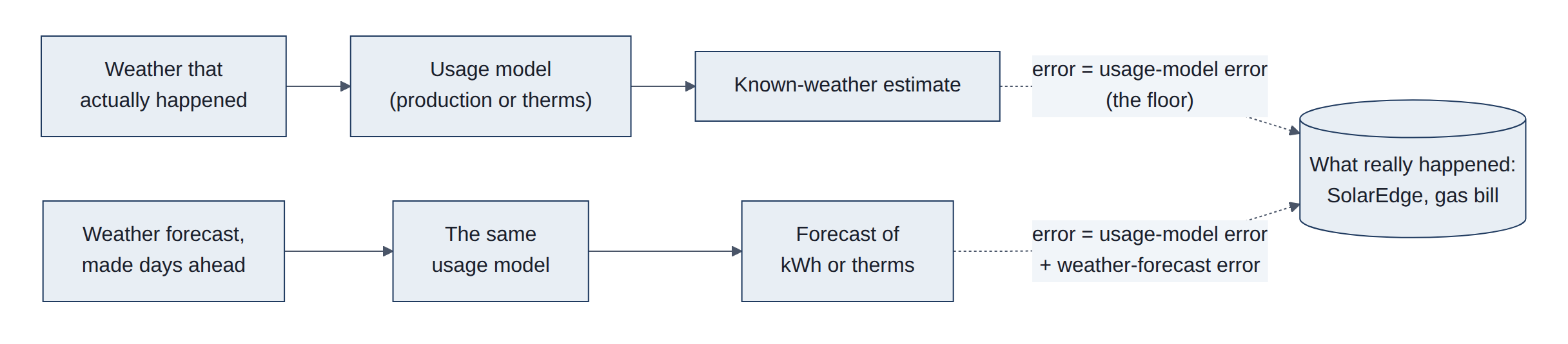
Shared code is verify._scores (bias, MAE, root mean square error (RMSE), MAE of each baseline and skill), which scores only cases where the forecast, the truth and every baseline exist, so all MAEs in a row describe the same cases. Ensemble coverage and calibration are in hdd.py. Results are recomputed on every fc page run, and the headline numbers are written to runs.jsonl. The intervals come from verify.block_means (a circular moving-block bootstrap using prefix sums, with a fixed seed) and verify.intervals, which returns *_lo and *_hi columns for each MAE and skill in a _scores table; energy.bill_intervals does the same for gas bills. Only scripts/snapshot_results.py computes them, so the daily page build is not slowed.
4.3.2 Temperature forecasts
The temperature check asks how good the NOAA forecasts are for this house, and for how many days ahead. Every stored run of the two models is compared with the house and airport stations hour by hour, and with PRISM for the daily high and low.
Views fc_verify_hourly and fc_verify_daily (sql/verify.sql).
- Hourly truth: station readings within 10 minutes of the hour.
- Hourly persistence: the latest same-hour observation known when the run started (valid time minus 24 h x ceil(lead / 24)).
- Hourly climatology: the 2015-2024 HRRR analysis mean for that week of the year and hour.
- Daily highs and lows: computed over the PRISM day (12:00 to 12:00 UTC); GFS uses its 6-hour maximum and minimum fields.
- Window: the last 90 days, both stations pooled.
4.3.3 Solar production: known weather and forecast
Production is estimated in three steps:
- Take the day's sunlight on flat ground.
- Convert it to what this tilted array should make, using the European Commission's Photovoltaic Geographical Information System (PVGIS) model of the exact system, month by month.
- Scale it by how the real array compares with that model.
With known weather, the sunlight comes from PRISM's measured value or from the HRRR analysis (NOAA's estimate of what happened). This measures the usage-model error. With a forecast, the same chain starts from the sunlight that HRRR or GFS predicted days earlier, and the result is scored against what the SolarEdge inverter recorded.
The forecasts are also compared with the two baselines:
- Persistence: the last full day's production.
- Normal: production in average 1991-2020 sunlight for the date.
Module solar.py, views in sql/solar_forecast.sql, page part in charts/solar_section.py.
- Solar day: 06:00 UTC on local day D to 06:00 UTC on D+1, which holds all of day D's sunlight. - HRRR sunlight is an instant at the top of each hour, so the day is the mean of 24 values. - GFS sunlight is a running mean from the last 6-hour boundary, so only the values at lead hours divisible by 6 are used: four 6-hour means. This also works where GFS steps every 3 hours. - A day counts only when every value is present.
- Lead day: D minus the run's Eastern date. Day 0 is the same day from a run made before sunrise; day 1 is tomorrow.
- Production model: kWh = k x PVGIS factor x daily sunlight, with sunlight in megajoules per square metre per day (MJ/m2/day) and the factor in kWh per MJ/m2. - The PVGIS factor is the PVGIS monthly kWh divided by PRISM's 1991-2020 mean monthly sunlight. - Since this version it is interpolated between mid-month values, removing a 40% step at the end of October. - The share k is fitted through the origin on all days since the array started, refitted without snow-flagged days.
- Sunlight scale: each model's daily sunlight runs above PRISM's (GFS by about 2%, HRRR forecast by 7-10%, HRRR analysis by about 4%), so it is divided by its ratio to PRISM. - The ratio is fitted on the other calendar months only, so the score is out of sample. - The live forecast uses the ratio over all scored days.
- Scoring: snow days stay in the score. The floors are scored on the same days as the forecasts.
4.3.4 Heating outlook and the gas bill
The house heats with a gas boiler, so cold weather means gas.
- Heating degree days (HDD) measure the cold: how far a day's mean temperature falls below 65 degrees Fahrenheit (degF), or 18.3 degC.
- Usage model: fitted on three years of gas bills, it turns degree days into therms of gas (one therm is about 29.3 kWh of heat).
- Forecast: NOAA's Global Ensemble Forecast System (GEFS) runs its model 31 times with slightly different starting points. The spread of the runs gives a range for the coming 35 days.
Two checks follow:
- Degree days: every daily GEFS run since October 2020 is compared with the degree days observed at the airport, in heating seasons (October to April).
- Gas bills: gas is metered only once a month, so the gas forecast can only be checked one bill at a time. - For each bill, every GEFS run from the 35 days before the meter read is replayed. - Days before the run use the degree days that were observed; days from the run on use that run's forecast. - The usage model, fitted only on earlier bills, turns the result into therms, which are compared with the bill. - The same days are also filled with normal weather, and with persistence (the last observed day repeated). - At 0 days before the meter read the weather is fully known, so that point is the usage-model error alone.
- Degree days:
hdd.py,sql/ensemble.sql. - Each member's daily mean is the mean of its 00, 06, 12 and 18 UTC temperatures; degree days are taken per member before summing windows. - Calibration (D14) shifts the centre by the mean past error and sets the spread to sqrt(c + d x ensemble variance), fitted per lead day or window. - In the back-test each heating season is calibrated on the other seasons only. - Gas bills:
energy.bill_forecastsandenergy.bill_scores. - A run starting on day R uses observed degree days before R and the calibrated daily median from R on. Lead = meter-read date minus R, from 0 to 35 days. - Bills since October 2021 with every day observed are used. The usage model isenergy.fit_gason bills ending before the one scored, as inbacktest_bills. - Errors are averaged per bill within weekly lead bins. Only bills scored in every bin are kept, so the bins compare the same bills. - Dollars use each bill's own volumetric rate.
4.3.5 Household electricity and net grid use
The electricity check asks how much electricity the house will use in the coming days, how much of it the solar panels will cover, and how good such forecasts have been.
The "actual" is the household's daily use, however it is supplied:
- Before the panels (until January 2026): the utility's billing meter measured all of it.
- Since the panels went in: use is what came from the grid, plus what the panels made, minus what went back to the grid.
- Recent days: the utility's data is downloaded by hand and lags by weeks, so for recent days the SolarEdge monitoring system's own figure is used. It is scaled up by 3%, the amount it reads below the meter.
The usage model is a change-point model, the standard way to relate a building's energy use to the weather. It comes from the Princeton Scorekeeping Method (Fels 1986), which is unrelated to the PRISM weather maps despite the shared name:
- Base load: a fixed amount of use per day.
- Heating: an extra amount for each degree the day's mean temperature falls below a balance point.
- Cooling: an extra amount for each degree above a second balance point (air conditioning).
- Weekends: a small extra amount.
Temperature explains only part of daily use; habits matter as much. The forecast therefore adds the household's recent level: how far above or below the model use has run over the past four weeks. Every past GEFS run since October 2020 is replayed through this model and scored against what the household actually used.
Three baselines apply:
- Persistence: the last day's use.
- Normal: the model fed 1991-2020 weather.
- Normal plus the recent level: this one shows what the weather forecast adds on top of simply knowing the household's habits.
Net grid use is use minus solar production: what the house draws from the grid, or sends to it when the number is negative. Its forecast combines the use forecast with the solar forecast of section 4.3.3, and covers the days with solar forecasts.
Module electric.py, page part charts/electric_section.py.
- Truth (
electric.consumption): - Beforecmp_tariff.SOLAR_COMMISSIONED:v_daily_electric.d_kwhon days with at least 23 hours. - After it: meter import + SolarEdge daily production - meter export. - Elsewhere:seh_power_details.consumption_wsummed over days with at least 92 quarter-hours, times the ratio of the meter route to SolarEdge over the days both exist (1.029). - Model: kWh = base + h x max(0, Th - T) + c x max(0, T - Tc) + w x weekend, with T the KPWM daily mean. - Th (25-65 degF) and Tc (55-75 degF, Tc >= Th) by grid search; the rest by least squares. - A negative slope is dropped and the fit repeated. - Refitted for every month on the 365 days before the month starts, so predictions are out of sample.
- Recent level: the mean of (actual - model) over the 28 days before the day predicted (at least 20 present), carried forward up to 3 days to cover SolarEdge sync lags.
- GEFS: - Members' daily means are shifted per lead day by the mean (observed - ensemble mean), fitted on the other seasons only, then put through the model of the run's month. - The forecast is the member mean plus the level. - The 80% range is the forecast +- 1.28 x sqrt(member variance + scatter^2), where scatter is the standard deviation of the level-adjusted known-weather error over the year before the run's month.
- Net: GEFS use minus the GFS 06 UTC solar forecast from the same date (
solar.frame), against actual use minus SolarEdge production. Baselines are the normal of each and the last day's net.
4.4 Current access: the wrapper
The wrapper is a small helper library from dynamical.org. Given a dataset name, it reads the catalog, works out where the data lives, opens the repository with the right settings, and returns the data ready to use. It retries when the catalog is briefly unreachable, checks that the catalog makes sense, and handles the extra setup that virtual datasets need. It is about 800 lines of code (Figure 22).
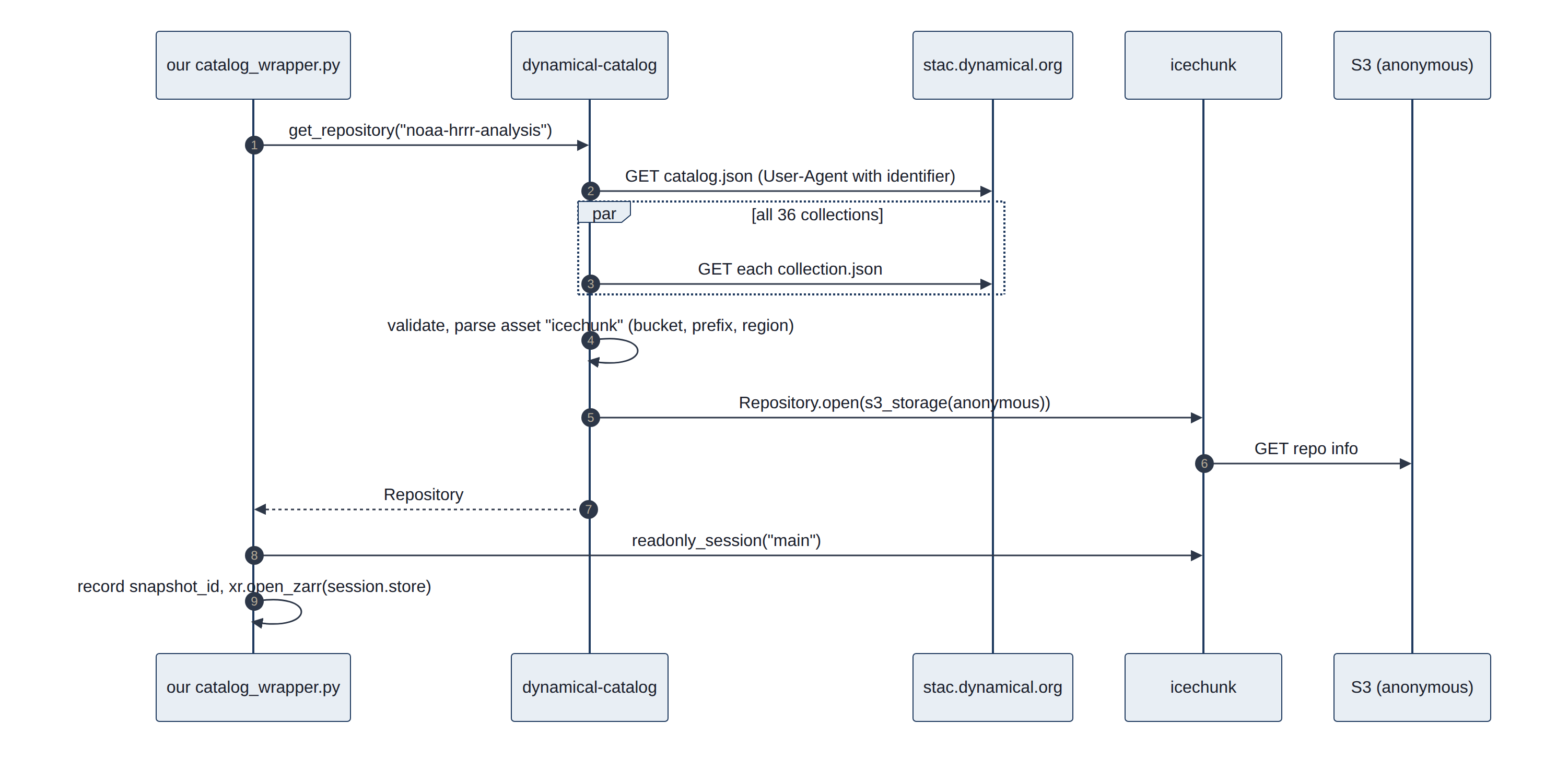
Read from dynamical-catalog 1.0.1 (__init__.py 176 lines, _open.py 111, _stac.py 420, exceptions.py 78) (Table 12):
Table 12. What the wrapper does at each step.
| Step | Wrapper behavior |
|---|---|
| Catalog fetch | load_catalog() fetches catalog.json, then every child Collection in parallel (ThreadPoolExecutor), caches the parsed result per process. If any one Collection fails, the whole load raises CatalogFetchError. Measured: 0.92 s for 36 Collections, against 0.10 s for one |
| HTTP | urllib, 10 s timeout, 3 attempts with 1 s backoff; retries 429, 409 and transient connection errors; fails fast on other 4xx and on invalid JSON |
| Identification | identify(email) appends (email) to the User-Agent dynamical-catalog/1.0.1 on catalog requests only |
| Override | DYNAMICAL_STAC_CATALOG_URL points at staging or test catalogs |
| Asset choice | Always the asset keyed icechunk (never icechunk-https) |
| Storage | Maps the href scheme to anonymous Icechunk storage: s3, gcs, azure, tigris, http; S3 and Tigris require xarray:storage_options.client_kwargs.region_name |
| Catalog validation | Rejects missing id/assets/icechunk asset, duplicate IDs, unknown schemes, and any virtual container that carries credential material or non-anonymous access |
| Virtual datasets | Builds containers_credentials from the Collection and passes it as authorize_virtual_chunk_access |
| Open | Repository.open(storage), then readonly_session("main").store, then xr.open_zarr(store, **kwargs) |
| Errors | Typed exceptions: UnknownDatasetError, CatalogFetchError, InvalidCatalogError, DatasetOpenError |
This project already bypasses one wrapper step: catalog_wrapper.py calls get_repository() and opens its own read-only session so it can record the exact snapshot ID next to the data (07-client-migration.md).
4.5 Alternative: direct access
Going direct means writing those steps ourselves: read the one catalog entry we need, connect to storage, open the repository at a known version, and open the arrays. Each step is a few lines with the underlying libraries. The work is not in the normal path; it is in deciding what to do when something is missing, slow or changed (Figure 23).
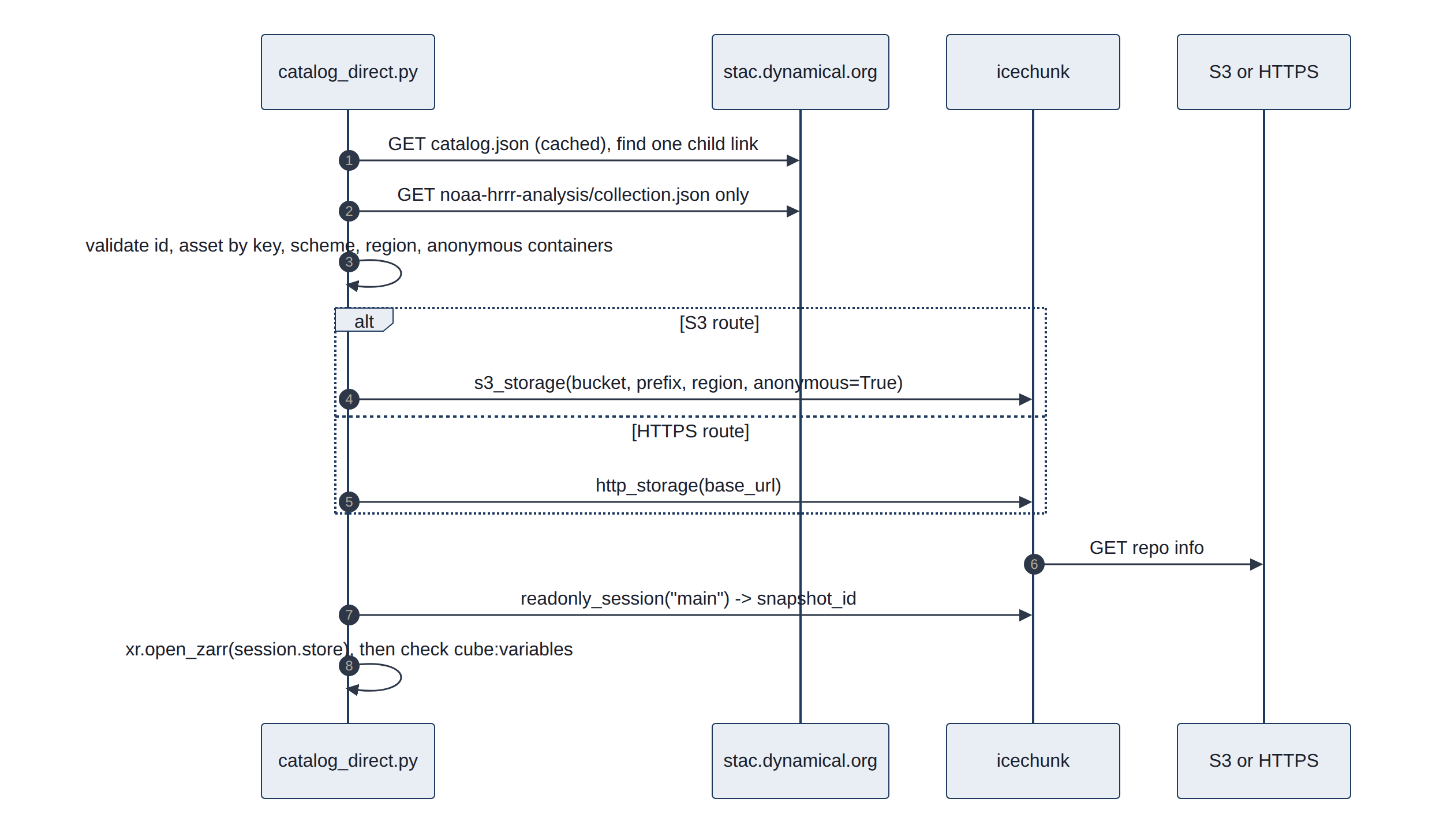
The direct client implements the four-function interface in catalog.py (open_dataset, get_repository, current_snapshot_id, list_datasets) (Table 13).
Table 13. Direct access for each piece, with the checks to add.
| Piece | Direct approach | Checks to add |
|---|---|---|
| Catalog | urllib GET of one Collection (find its href from the catalog's child links); pystac optional and not installed | id matches; assets.icechunk present; scheme in allow-list (s3, https); region present for S3; containers anonymous-only; User-Agent with DYNAMICAL_IDENTIFY_EMAIL |
| Asset | Choose by key (icechunk or icechunk-https) | Phase 0 found "first asset containing icechunk" picked the s3:// asset, which http_storage rejects |
| Repository | icechunk.s3_storage(bucket=, prefix=, region=, anonymous=True) or icechunk.http_storage(base_url=); Repository.open(storage, authorize_virtual_chunk_access=...) only when containers are listed | Measured: both routes opened the same snapshot and returned identical values |
| Session | readonly_session("main"); record session.snapshot_id; readonly_session(snapshot_id=...) for re-reads | |
| Arrays | xr.open_zarr(session.store, chunks=None, consolidated=False): Icechunk has no consolidated metadata; chunks=None stays lazy without Dask | Compare against cube:variables and dynamical-org:chunking to fail early on renamed variables or a changed layout |
| Virtual (only if adopted) | icechunk.containers_credentials({prefix: icechunk.s3_anonymous_credentials()}) per listed container | Keep gribberish installed: without it, reads fail at decode time, not at open time |
5. Results
5.1 Station checks
Each station's average offset from PRISM, by year, is summarised below (station minus PRISM, in degrees Fahrenheit; a positive number means the station reads warmer). The subsections then take the stations one at a time (Table 14).
Table 14. Station offsets against PRISM by year, with verdicts.
| Station | Daily highs vs PRISM | Daily lows vs PRISM | Verdict |
|---|---|---|---|
| KPWM | -0.3 to +0.1 (2017-2023), about -0.7 (2024-2026) | -0.3 to +0.4 (2017-2023), about -0.4 to -0.8 (2024-2026) | Reliable reference; small step in 2024, cause not identified |
| ZASTMET | +1.8 (2024), +1.4 (2025), +0.6 (2026) | -0.5 (2024), 0.0 (2025), -0.8 (2026) | Reads cooler each year: drift, see below |
| E4229 | +0.5 to +1.3 (2017-2019), +4.8 to +6.8 (2020-2026) | +6.4 to +8.4 (2020-2021), wrecked from 2022 (placeholder zeros) | Excluded from all analyses since 2026-10-27 |
| E4279 | within 1 degree | -1.3 to -4.2 (2017-2022), within 0.7 since 2024 | Usable since 2024 |
| G5290 | within 0.5 since 2025 | -1.7 to -2.7 | Reads cold at night |
| G5544 | about -0.5 | about -0.5 | Good temperature; wind sensor dead |
5.1.1 KPWM: Portland International Jetport
KPWM is the official National Weather Service station at the airport, 19 m above sea level near the coast. It is an ASOS (Automated Surface Observing System), the standard US airport station. Its thermometer sits in a shield with a fan that pulls outside air past it (an aspirated shield), so sunshine cannot warm it, and technicians maintain and calibrate it. It reports once an hour, just before the hour (at :51), plus extra reports when the weather changes quickly. It is the most trustworthy station here and the one used for heating degree days, the gas usage model and the heating outlook.
Two cautions. First, because it reports only hourly, its daily high and low can miss a short peak between reports, so they read slightly less extreme than a station sampling every 5 minutes. Second, NOAA's models and PRISM both use KPWM as an input, so KPWM agreeing with them proves less than ZASTMET agreeing with them.
ASOS measures dry-bulb temperature with a platinum resistance thermometer in an aspirated air stream at about 1.5 m, and dew point with a dedicated hygrometer (National Weather Service (NWS) ASOS, ASOS temperature and dew point sensor). Rows come from METAR reports via Gladstone into wx.KPWM (dt_utc, temp_f, dewpoint_f, humid_perc, pressure_mbar, windsp_mph, windir_deg). Measured offset against HRRR, by quarter: -0.5 to +0.8 degF since 2021, with larger values (+1.4 to +2.5) in several quarters of 2019-2020. The -0.7 degF step against PRISM since 2024 appears in highs and lows alike; PRISM's own station inputs and methods change over time, so the cause may be on either side.
5.1.2 ZASTMET: the house station (Ambient Weather WS-2902)
ZASTMET is the owner's own station at the house, an Ambient Weather WS-2902. It is an all-in-one sensor unit on a pole: thermometer and humidity sensor inside a stack of white plates (a passive radiation shield, with no fan), wind cups and vane, a rain gauge that counts small tips of a bucket, and a light sensor for sunshine and ultraviolet (UV) light. It is solar powered and sends its readings by radio to a console indoors, which posts them to ambientweather.net every few minutes. The project reads them from there, one reading every 5 minutes.
Ambient states the thermometer is accurate to within 2 degF and the light sensor to within 15%. Both limits show up in our data:
- Sunshine reads low. The light sensor measures brightness and converts it to solar power with a fixed factor. Against PRISM's satellite-based sunshine it reads about 27% low (PRISM is 1.37 times the house value, over 484 days), so the solar charts scale it before use.
- Sunny-day warmth. Without a fan, the shield warms in strong sun and light wind. In 2024 and 2025 the house's daily highs ran 1.4 to 1.8 degF above PRISM, while its lows were close.
- Temperature drift since December 2025. Compared with the HRRR analysis, the house station read about 0.5 to 1 degF warmer through 2024 and most of 2025. From December 2025 it has read 0.3 to 1.4 degF colder: a swing of about 2 degF. The airport station, compared with the same HRRR grid over the same months, did not move, so the change is at the house station and not in the model. PRISM shows the same thing: the house's highs fell from 1.8 to 0.6 degF above PRISM, and its lows from 0.0 to 0.8 degF below.
Figure 24 shows the monthly offset against the HRRR analysis.
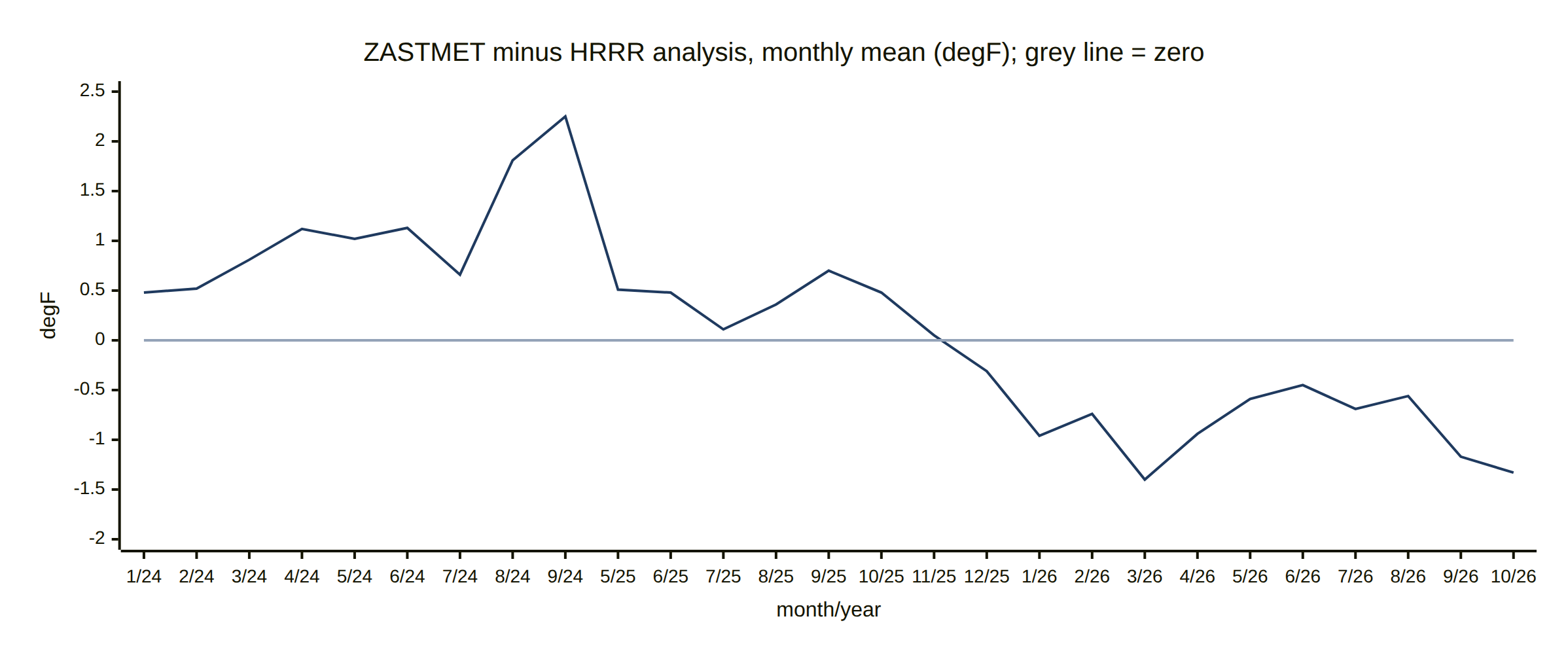
Each point is one month; the station was offline from mid-September 2024 to May 2025, so those months are missing: the axis jumps from 9/24 (September 2024) to 5/25 (May 2025). Possible causes worth checking at the station: a dirty or cobweb-filled shield, a sensor that is aging, a change in mounting height or surroundings (new shade, a nearby surface that warms or cools), or a low battery. A side-by-side check with a trusted thermometer for a few days would settle it. The station checks chart on the results page tracks this offset every day.
Table wx.zastmet: dateutc (epoch seconds, converted with to_timestamp), tempf, humidity, dewPoint, solarradiation (watts per square metre, W/m2, derived from lux), uv, wind, rain counters, indoor values (tempinf, humidityin), pressure (baromrelin, baromabsin) and battout. Readings per day rose from about 195 (2024) to 288 (2026), so a day counts as complete with readings in 22 of 24 hours. The pyranometer factor (1.37 to PRISM, 1.45 to HRRR) is recomputed on every page build. The stations table lists the equipment as a WS-2000; the owner reports a WS-2902, which this document uses.
Monthly ZASTMET minus HRRR (degF, hours with at least 3 readings): 2024: +0.5, +0.5, +0.8, +1.1, +1.0, +1.1, +0.7, +1.8, +2.3 (Jan-Sep); 2025: +0.5, +0.5, +0.1, +0.4, +0.7, +0.5, +0.1, -0.3 (May-Dec); 2026: -1.0, -0.7, -1.4, -0.9, -0.6, -0.5, -0.7, -0.6, -1.2, -1.3 (Jan-Oct).
5.1.3 The volunteer (CWOP) stations
CWOP stations belong to private volunteers who share their readings with NOAA. They fill the gaps between official stations, but quality varies and nobody checks the hardware. Their main use here is to compare with each other and with PRISM, and to show what a faulty station looks like.
- E4229 (Cumberland, 64 m): no longer used. Two serious problems led to its removal from every analysis on 2026-10-27 (its readings are still collected). Since 2020 its daily highs have run about 5 to 7 degF above PRISM, and in 2020-2021 its lows ran 6 to 8 degF above too (before 2020 both were within about 1 degF). That suggests the sensor was moved, re-shielded or sits in a warm spot. Since 2022, about one reading in eight has temperature, dew point and humidity all exactly 0 while pressure keeps reporting: these are placeholders for missing readings, not real cold. They drag daily lows down by more than 30 degF and pull daily and weekly averages cold. Five readings of -90 degF in 2024 are also errors. The main site's charts had already dropped it in July 2026; the forecasting PRISM checks, the data quality report and the analysis notebook dropped it on 2026-10-27.
- E4279 (Gray, 96 m, Davis Vantage Pro2). A well-known hobbyist station design (Davis Vantage Pro2). Its lows ran 1.3 to 4.2 degF below PRISM in 2017-2022 and are within 0.7 degF since 2024. MADIS notes its dew point has larger errors than usual. It was offline from February to November 2025.
- G5290 (Yarmouth, 30 m). Daily lows run 1.7 to 2.7 degF below PRISM, and MADIS flags its temperature as reading cold. Its low site near the coast may collect cold air on calm nights (cold air pooling), a real local effect rather than a fault, but it makes the station unrepresentative of the wider area.
- G5544 (Freeport, 55 m). Temperature agrees with PRISM to about 0.5 degF and MADIS passes all its sensors, but its average wind speed over the last year is 0.04 mph: the anemometer is stuck or fully sheltered.
CWOP tables share the schema dt_utc, temp_f, dewpoint_f, humid_perc, pressure_mbar, windsp_mph, windir_deg (plus a_* columns). E4229 placeholder rows match temp_f = 0 AND dewpoint_f = 0 AND humid_perc = 0 (11 to 15% of rows per year since 2022, and 7 to 16% in every month including summer, so they cannot be real cold). The station was removed from PRISM_SITES (forecasting), HOURLY_STATIONS (data_quality_report.py) and the marimo notebook; fetchweather.sh and the Snowflake push still collect it, and its v_E4229_* views remain in MariaDB. All four CWOP stations share a collection gap from 2025-02-12 to 2025-03-12 and a short one around 2026-01-01, which are download outages rather than station faults. PRISM daily values are loaded for the five sites in use (fc_prism_daily; E4229's earlier rows remain on disk but are no longer updated), but only ZASTMET and KPWM have L2 model point tables (D3).
5.2 Cloud-native versus traditional access
The traditional way to get NOAA model data is to download NOAA's files: one per model run per forecast hour, each covering the whole country with every variable. A year of hourly temperature at the house means thousands of files. The cloud-native form is arranged as time series, so the same year is a handful of small reads, with no NOAA server to queue behind, and a version history that makes results repeatable (Figure 25).
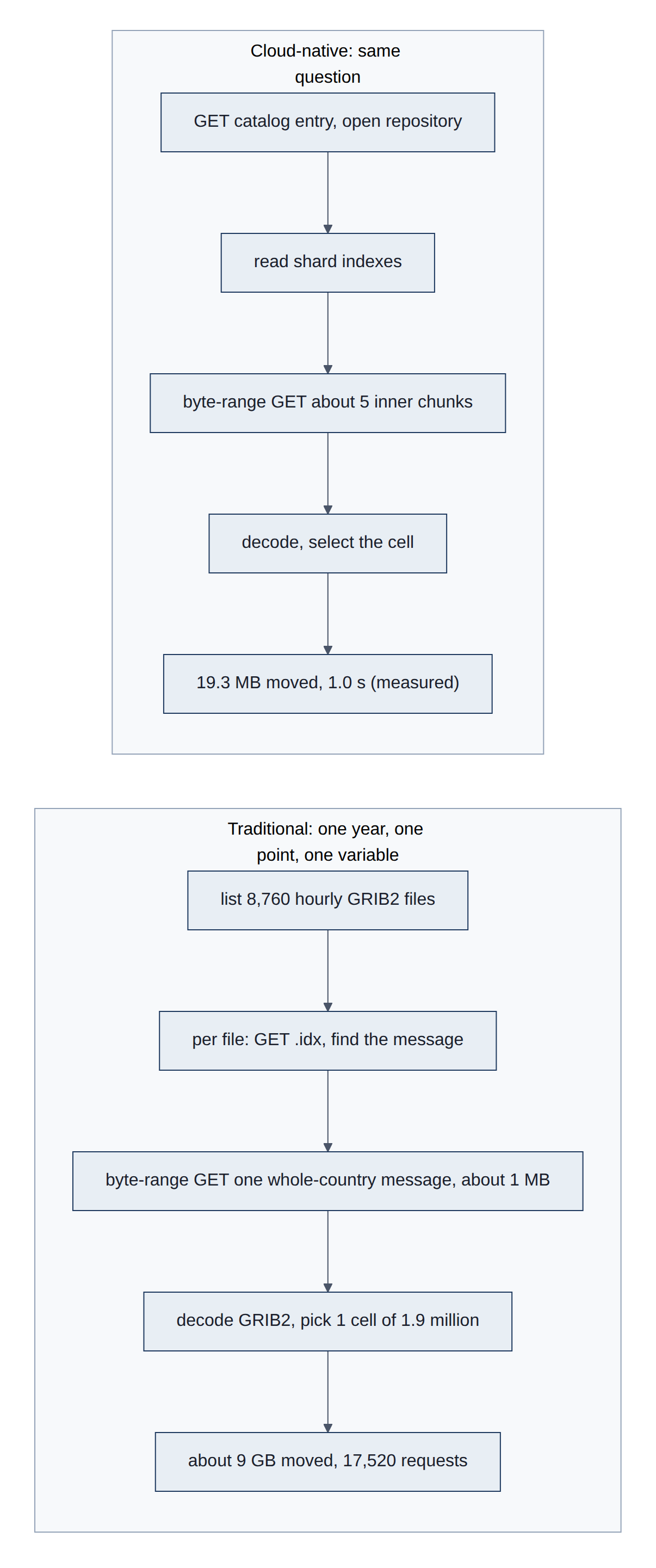
Table 15 compares the two routes concern by concern.
Table 15. Traditional versus cloud-native access, concern by concern.
| Concern | Traditional (NOMADS / NODD GRIB2, THREDDS/OPeNDAP) | Cloud-native (STAC + Icechunk + Zarr) |
|---|---|---|
| Unit of access | One GRIB2 file per run and forecast hour (HRRR surface files are roughly 100-150 MB) | Byte ranges for the chunks touched |
| One variable, one point, one year of HRRR analysis | 8,760 files; even with .idx byte-range reads, one ~1 MB compressed message per hour covering the contiguous United States (CONUS), around 9 GB | Measured: 19.3 MB, 1.0 s |
| Server | NOMADS rate limits and a short retention window; THREDDS/OPeNDAP depends on a live server | Static objects on S3; no server logic, scales with the object store |
| History | The NOAA Operational Model Archive and Distribution System (NOMADS) keeps days; archives (National Centers for Environmental Information, NCEI; NOAA Open Data Dissemination, NODD) are file collections with gaps to stitch | One continuous store from 2014, gaps marked as NaN |
| Consistency | Files appear one by one; a reader can see a half-published run | Snapshot isolation: a read sees a whole commit or none |
| Reproducibility | No version identity beyond file names; re-runs and corrections overwrite | Snapshot IDs; old snapshots stay readable |
| Decoding | wgrib2 / cfgrib / eccodes, grid-relative winds, accumulations to de-accumulate | Decoded floats with units and CF attributes; precipitation already as rates |
| Discovery | Directory listings and documentation | Machine-readable STAC with variables, extents and chunking |
The costs are real too: the layout favors time series (a full-country map at one hour touches many shards), values are lossy-rounded, and the service is a young non-profit (05-risks-security-decisions.md). For this project's access pattern the trade is strongly favorable.
5.3 Forecast checks
All five forecasts beat both simple guesses at short lead times, and each stops being useful at a different horizon. Temperature and sunshine forecasts are clearly useful for about 5 days (on average for about a week), and the cold (degree days) for about two weeks. For the gas bill and for household electricity, the weather forecast is not the main source of error: the usage model and household habits are. The subsections give the numbers, as of the 2026-10-27 page build.
5.3.1 Temperature
Forecasts for the next few hours miss the hourly temperature at the house and the airport by about 2 degF (1.1 degC). Both models beat "same as yesterday" by a wide margin on day 2. GFS is clearly better than the normal (95% bootstrap interval of skill above zero, section 4.3.1) through day 5 for both highs and lows; on average it stays ahead to day 6 for highs and day 8 for lows (Table 16).
Table 16. Temperature forecast error, last 90 days (degF; 1 degF = 0.56 degC).
| Measure | HRRR | GFS | Persistence |
|---|---|---|---|
| Hourly MAE, lead 1-6 hours | 1.9 | ||
| Hourly MAE, day 2 (lead 25-48 hours) | 2.7 | 2.9 | 6.2 |
| Last day GFS beats the normal on average, daily high | day 6 | ||
| Last day GFS beats the normal on average, daily low | day 8 | ||
| Last day GFS clearly beats the normal (95%), highs and lows | day 5 |
5.3.2 Solar production
The array averaged 47 kWh a day over the scored period.
- Tomorrow: the GFS forecast missed by 7 kWh on average (15%). Guessing the normal missed by 17 kWh, and repeating the last day by 22 kWh.
- Lead time: the error grows steadily with lead time. GFS is clearly better than the normal through day 5, better on average through day 7, and worse from day 8 (Table 17).
- HRRR: NOAA's 3 km model is no better than GFS for daily solar totals on days 0 and 1.
- Floor: even with the actual sunlight known, the production model misses by 4.3 kWh (PRISM sunlight) or 5.7 kWh (HRRR analysis). So about 3 of tomorrow's 7 kWh of error come from forecasting the weather, and the rest is the usage-model error.
Over all 271 days since the array started, including the winter snow days, the floors are 4.5 kWh (PRISM) and 7.7 kWh (HRRR analysis). With smooth daily conversion factors, the known-weather model explains production with r = 0.970 and a typical daily error of 7.8% (excluding the 7 snow days).
Table 17. Solar production forecast error by lead day, 2026-07-29 to 2026-10-24 (kWh per day; mean production 47 kWh per day).
| Source | Lead day | Days scored | Bias | MAE | MAE, normal | MAE, persistence | Skill vs normal |
|---|---|---|---|---|---|---|---|
| PRISM sunlight (known weather) | 88 | -1.0 | 4.3 | 16.9 | 20.0 | 0.75 | |
| HRRR analysis (known weather) | 88 | -0.4 | 5.7 | 16.9 | 20.0 | 0.66 | |
| HRRR forecast | 0 | 88 | +0.4 | 7.2 | 16.9 | 20.0 | 0.57 |
| HRRR forecast | 1 | 350 | -1.0 | 7.9 | 16.8 | 21.5 | 0.53 |
| GFS forecast | 0 | 88 | +0.5 | 7.0 | 16.9 | 20.0 | 0.59 |
| GFS forecast | 1 | 351 | -0.1 | 7.0 | 16.9 | 21.6 | 0.59 |
| GFS forecast | 2 | 347 | -0.5 | 7.8 | 16.8 | 20.8 | 0.53 |
| GFS forecast | 3 | 343 | -1.5 | 9.5 | 16.9 | 21.1 | 0.44 |
| GFS forecast | 5 | 335 | -0.2 | 14.0 | 17.1 | 23.6 | 0.18 |
| GFS forecast | 7 | 327 | -0.6 | 16.5 | 16.9 | 22.8 | 0.02 |
| GFS forecast | 8 | 323 | -0.8 | 20.3 | 17.0 | 22.1 | -0.20 |
| GFS forecast | 14 | 299 | -1.1 | 23.2 | 17.6 | 19.5 | -0.32 |
"Days scored" counts run-day pairs: four runs a day each forecast the same day.
5.3.3 Heating degree days
Over six heating seasons, the GEFS forecast of next week's total degree days missed by 10 HDD on average, against 27 for the normal and 41 for persistence. At current prices 10 HDD is about $4 of heating.
- Daily forecasts: they are clearly better than the normal through day 13: there the lower end of the 95% bootstrap interval of their skill (section 4.3.1) is above zero. Their average stays slightly ahead to about day 26, but by too little (skill at most 0.05) to tell apart from the normal.
- Raw ranges: too narrow, holding the actual week only 55% of the time.
- Calibrated ranges: they held it 81% of the time (77% for the following week), close to the 80% target, while staying about a third as wide as the range of normal weather.
5.3.4 Gas bills forecast ahead
Forty-six bills, from October 2021 to August 2026, were scored (Table 18).
- All bills, weather known: the usage model misses by 22% per bill on average. Most of that comes from summer bills, which are small and in 2026 about double the model's base use.
- All bills, a month ahead: forecast 29 to 35 days before the meter read, when almost the whole bill is still in the future, the error rises only to 24%. Normal weather gives 29% and persistence 39%.
- Winter bills (starting November to February, 15 bills): the usage model alone misses by 6%, and a month-ahead forecast also by 6%, against 11% for normal weather and 21% for persistence.
In dollars, at each bill's own rate, a month-ahead forecast is off by about $28 per bill, against $37 for the normal. The GEFS forecast clearly beats both baselines beyond a week. The usage model, not the weather forecast, limits the bill forecast.
Table 18. Gas bill forecast error by days before the meter read (mean absolute error per bill, % of billed therms).
| Days before meter read | Share of bill days forecast | GEFS, all 46 bills | Normal, all | Persistence, all | GEFS, 15 winter bills | Normal, winter | Persistence, winter |
|---|---|---|---|---|---|---|---|
| 0 (weather known) | 0% | 22.0 | 22.0 | 22.0 | 5.7 | 5.7 | 5.7 |
| 1-7 | 13% | 21.6 | 22.7 | 21.3 | 5.3 | 6.9 | 5.8 |
| 8-14 | 36% | 21.4 | 24.6 | 24.3 | 5.9 | 8.4 | 9.7 |
| 15-21 | 59% | 22.0 | 26.4 | 27.4 | 8.1 | 8.7 | 11.9 |
| 22-28 | 82% | 23.2 | 27.5 | 33.5 | 6.9 | 9.3 | 18.2 |
| 29-35 | 98% | 24.3 | 29.1 | 38.8 | 5.8 | 10.9 | 20.8 |
5.3.5 Household electricity and net grid use
The house uses about 42 kWh a day on average. The current model, fitted on the past year, has three parts:
- Base: 39 kWh a day.
- Cooling: 1.5 kWh for each degree the daily mean rises above 60 degF (15.6 degC), the largest weather effect, from air conditioning.
- Cold: 0.8 kWh for each degree below 38 degF (3.3 degC), and 2.2 kWh more on weekends.
Temperature explains only part of the day-to-day swing (r = 0.61), and the typical scatter around the model is 10 kWh a day.
The forecast results, over every GEFS run since October 2020 (Table 19):
- Tomorrow: the forecast misses by 7.6 kWh, against 9.5 kWh for the normal and 9.1 kWh for repeating the last day.
- Weather versus habits: most of that gain comes from the recent level. The normal plus the recent level misses by 8.0 kWh, so the weather forecast adds about 0.4 kWh a day in the first week and nothing beyond two weeks.
- Even with the weather known: the model with the actual temperature still misses by 7.5 kWh (9.1 kWh without the recent level). For the current day, repeating yesterday (7.4 kWh) is as good as any model.
- Weekly totals: for a typical week of 293 kWh, the coming week's forecast misses by 37 kWh (12%), against 51 kWh for the normal and 52 kWh for persistence.
- Range: the 80% range held the actual day 83% of the time.
Net grid use, over the 88 days with solar forecasts (2026-07-29 to 2026-10-24), averaged a draw of 3.5 kWh a day (Table 20). Tomorrow's net forecast misses by 9.9 kWh, against 17.1 kWh for normal weather. It is clearly better than the normal through day 4, better on average through day 5, and worse from day 7. That is the horizon of the solar forecast: cloud cover, not household use, limits the net forecast.
Table 19. Household electricity forecast error by lead day, every GEFS run 2020-10-01 to 2026-10-27 (kWh per day; mean use 42 kWh per day).
| Lead day | Days scored | Bias | MAE, GEFS + level | MAE, normal + level | MAE, normal | MAE, persistence | Skill vs normal | Skill vs normal + level |
|---|---|---|---|---|---|---|---|---|
| Known weather | 2,105 | 7.5 | 7.9 | 9.5 | 7.4 | 0.20 | 0.05 | |
| 1 | 2,101 | -0.4 | 7.6 | 8.0 | 9.5 | 9.1 | 0.19 | 0.05 |
| 3 | 2,094 | -0.4 | 7.8 | 8.2 | 9.5 | 9.8 | 0.18 | 0.05 |
| 7 | 2,083 | -0.1 | 8.0 | 8.4 | 9.7 | 10.2 | 0.17 | 0.05 |
| 14 | 2,069 | -0.2 | 8.6 | 8.7 | 9.8 | 11.0 | 0.12 | 0.01 |
| 21 | 2,055 | 0.0 | 8.8 | 8.8 | 9.9 | 11.1 | 0.11 | 0.00 |
| 34 | 2,032 | +0.3 | 9.1 | 9.2 | 10.0 | 11.7 | 0.10 | 0.01 |
| Week, days 0-6 (total) | 2,021 | -2.3 | 36.6 | 39.0 | 51.1 | 51.8 | 0.28 | 0.06 |
| Week, days 7-13 (total) | 2,000 | -1.1 | 41.6 | 43.3 | 52.8 | 60.6 | 0.21 | 0.04 |
The known-weather row uses the observed temperature; its MAE columns score the same days.
Table 20. Net grid use forecast error by lead day, 2026-07-29 to 2026-10-24 (kWh per day; GEFS use minus GFS solar).
| Lead day | Days scored | Bias | MAE | MAE, normal | MAE, persistence | Skill vs normal |
|---|---|---|---|---|---|---|
| 0 | 84 | -1.9 | 9.4 | 16.8 | 20.4 | 0.44 |
| 1 | 83 | -1.2 | 9.9 | 17.1 | 22.3 | 0.42 |
| 2 | 82 | -1.4 | 11.5 | 16.8 | 23.2 | 0.32 |
| 3 | 81 | -0.9 | 12.3 | 16.9 | 22.8 | 0.27 |
| 5 | 79 | -1.4 | 15.1 | 17.3 | 24.9 | 0.13 |
| 7 | 77 | +1.4 | 18.6 | 16.9 | 24.3 | -0.10 |
| 10 | 74 | +0.9 | 24.5 | 16.5 | 24.1 | -0.48 |
| 14 | 70 | +3.6 | 23.1 | 16.9 | 19.3 | -0.37 |
6. Discussion
6.1 Virtues of direct access
Doing it ourselves means understanding every step, which is the learning goal of this project. It removes a middleman whose choices we do not control, reads only what we need, and makes the cloud-native pieces visible rather than hidden behind one function call (Figure 26).
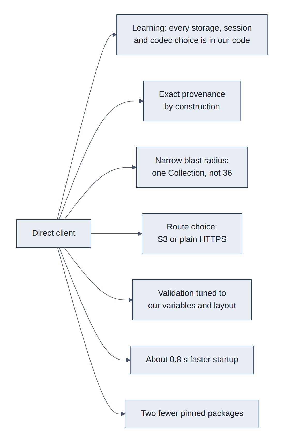
- Learning and transparency: every storage, session and codec decision is in our code and documented; that is the stated purpose of D7.
- Exact provenance by construction: session and snapshot are first-class, rather than worked around (today's
get_repository()detour). - Narrower blast radius: fetching one Collection means a broken or slow unrelated Collection cannot fail our run, which the wrapper's all-or-nothing
load_catalog()can. - Choice of route: HTTPS (
http_storage) avoids S3 signing logic entirely and works through plain HTTPS egress; S3 keeps region-aware access. The wrapper always uses theicechunkasset. - Tighter validation for our needs: check exactly the variables, units and chunking we rely on.
- Startup: about 0.8 s less per process (measured 0.10 s vs 0.92 s catalog load).
- One fewer pinned package:
dynamical-catalog(andgribberish, while no virtual dataset is used) leave the lockfile.
6.2 Downsides of direct access
We would own code that someone else currently maintains for us. When dynamical.org changes how their catalog or storage is described, their library is updated by the people making the change; ours would break until we noticed and fixed it (Figure 27).
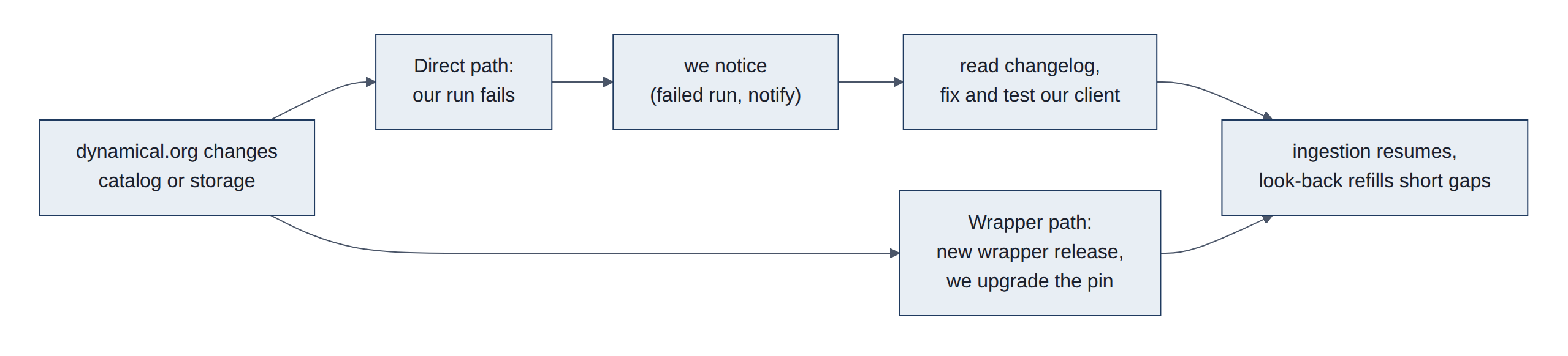
- Coupling to the catalog schema: asset keys,
xarray:storage_optionslayout, virtual container fields and theicechunk:extension names are dynamical.org conventions, not STAC core. The wrapper tracks them in lockstep; we would track them by reading changelogs. - Re-implementing robustness: retries with backoff on 429/409, timeouts, typed errors, and catalog validation (including the "no credential material" rule) must be rebuilt and tested.
- Storage backends: the wrapper handles S3, Google Cloud Storage (GCS), Azure, Tigris and HTTP; we would support only what we use (S3 and HTTPS) and fail on anything else. Fine today, a surprise later.
- Virtual datasets: authorization and codec registration are easy to get subtly wrong.
- Lost upstream fixes: wrapper releases may fix bugs we would have to discover ourselves.
- Identification: the User-Agent convention must be reproduced so dynamical.org's usage statistics still attribute traffic correctly.
6.3 Trade-offs: direct versus wrapper
Both read the same data at the same speed. The wrapper is less work and is kept current by the data's publisher; direct is more work and teaches more. Because the data is identical either way, the choice can be changed at any time with a single setting (Figure 28).
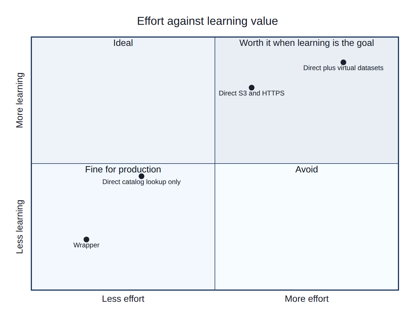
Table 21 compares the two options factor by factor.
Table 21. Wrapper versus direct access, factor by factor.
| Factor | Wrapper (current) | Direct |
|---|---|---|
| Values read | Identical (measured, same snapshot) | Identical |
| Open time | 1.50 s (measured, catalog cached) | 1.53 s |
| Process startup | +0.92 s catalog load | +0.10 s |
| Bytes transferred for data | Same | Same |
| Code we own | ~30 lines (catalog_wrapper.py) | ~150-250 lines plus tests |
| Upstream schema changes | Absorbed by the wrapper's maintainers | Ours to detect and fix |
| Failure isolation | One bad Collection fails every dataset | Only the Collection we read |
| Storage backends | Five | Two (S3, HTTPS) |
| Virtual datasets | Supported | Extra work if needed |
| Dependencies | dynamical-catalog 76 KB + gribberish 1.9 MB (in a 696 MB environment) | Neither, unless virtual datasets are used |
| Learning value | Low: one call hides the stack | High: the point of D7 |
| Reversibility | FC_CATALOG_CLIENT=direct | FC_CATALOG_CLIENT=wrapper |
Neither choice affects stored data: the local cube and Parquet tables are the same whichever client read them, and each commit records the client used.
6.4 Costs of switching
Switching is roughly two to three days of focused work, mostly testing and the side-by-side comparison, plus a little ongoing attention whenever dynamical.org changes their catalog. Running costs (time, data, money) do not change: the service is free and the amount downloaded is the same (Figure 29).
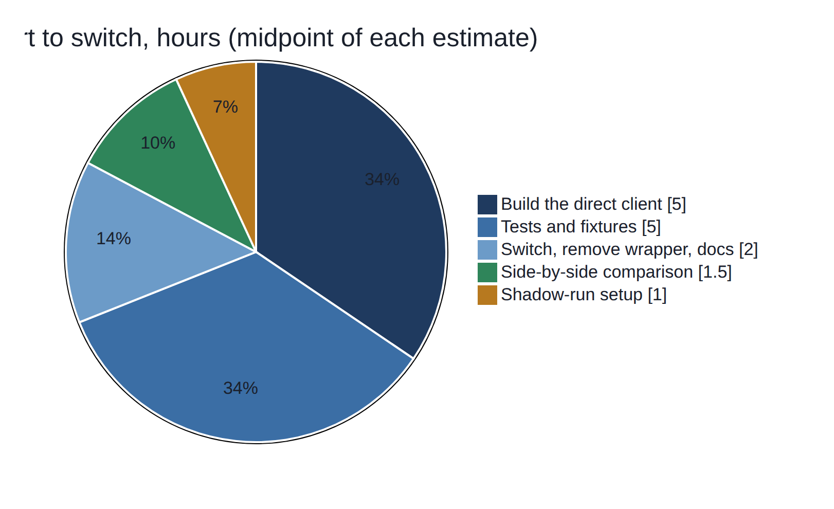
Figure 30 shows how the work could be scheduled if the decision is reopened.
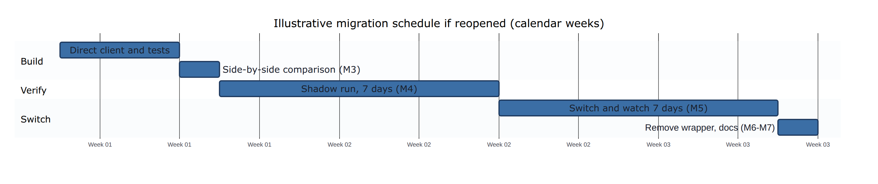
Table 22 lists each cost with its basis.
Table 22. Cost estimates for switching to direct access.
| Cost | Estimate | Basis |
|---|---|---|
Build catalog_direct.py (S3 and HTTPS routes, validation, retries, User-Agent) | 4-6 h | Appendix A sketch; wrapper logic is known (section 4.3) |
| Tests (shared interface tests parametrized by client; malformed catalog cases; offline fixtures of a Collection JSON) | 4-6 h | Existing test_safety.py pattern |
| Comparison M3 (identical values, metadata, snapshot; timing) | 1-2 h | Phase 0 script already did this once |
| Shadow run M4 (7 days into a throwaway cube) | 1 h setup, 7 days elapsed | fc_update.sh pattern |
| Switch, remove wrapper, re-lock, docs (M5-M7) | 2 h | |
| Total effort | about 12-17 h over 2-3 weeks elapsed | |
| Ongoing maintenance | ~1-2 h per catalog schema change; watch the dynamical.org updates feed | Unknown frequency; the service is young |
| Runtime, transfer, money | None added; about 0.8 s faster startup | Measured |
| Risk cost | A missed schema change stops ingestion until fixed; the cube keeps prior data and the look-back refills short gaps | 03-architecture.md failure handling |
6.5 Limitations
Some caveats apply. The references used to check stations are not fully independent: NOAA's HRRR model and the PRISM maps both use the airport station, and probably some volunteer stations, as inputs. PRISM revises each day's map for six months, so recent comparisons can shift slightly. The house station's record is short (since 2024, with an eight-month gap). The access timings were measured once, on one day, from one server, and would vary with network conditions. The solar forecast checks cover only 90 days of late summer and autumn, with no snow, so winter scores may differ. The production model's share of the PVGIS model is fitted on the same days it is checked on, which flatters the known-weather floor slightly. The gas checks rest on 46 bills, only 15 of them in winter, so the winter percentages can move by a few points as bills are added. The electricity model uses the airport's temperature, not the house's, and cannot see appliances or visitors; the net grid scores cover the same 90 autumn days as the solar scores. None of these changes the conclusions, but they limit how precisely the numbers should be read.
Independence: see section 4.2 and 08-phase0-results.md section 7. PRISM revisions: grids are stored with their release number (D10, D11), and scores quote the latest release. Station offsets use days with readings in at least 22 of 24 hours. The 19.3 MB / 1.0 s figure is one cold read of one variable at one cell for one year on 2026-10-26 (08).
7. Conclusions and recommendation
Four conclusions follow from this report:
- Cloud-native formats make this project practical: a year of hourly data at one place is a one-second read instead of a multi-gigabyte download (section 5.2).
- Station data needs continuous checking. The house station has drifted about 2 degF colder since December 2025, and E4229 was removed from all analyses for recording missing readings as zeros (section 5.1).
- Every forecast on the results page is shown with its own track record, which is what makes it usable for decisions such as the heating outlook. Temperature and sunshine forecasts are clearly better than the normal for about 5 days and degree days for about two weeks. For solar production about half of tomorrow's error is the weather forecast and half the production model. For gas bills the usage model, not the weather forecast, is the limit. Household electricity follows habits more than weather: tracking the recent level of use matters more than the temperature forecast, and net grid use is predictable only as far ahead as the sunshine (section 5.3).
- For the open design decision, the helper library is the right choice for now (below).
Stay on the wrapper, as decided. It works, it is maintained by the publisher, and switching would not change a single number. Revisit when there is a concrete reason: a problem the wrapper causes, a feature it lacks, or time set aside for the learning exercise (Figure 31).
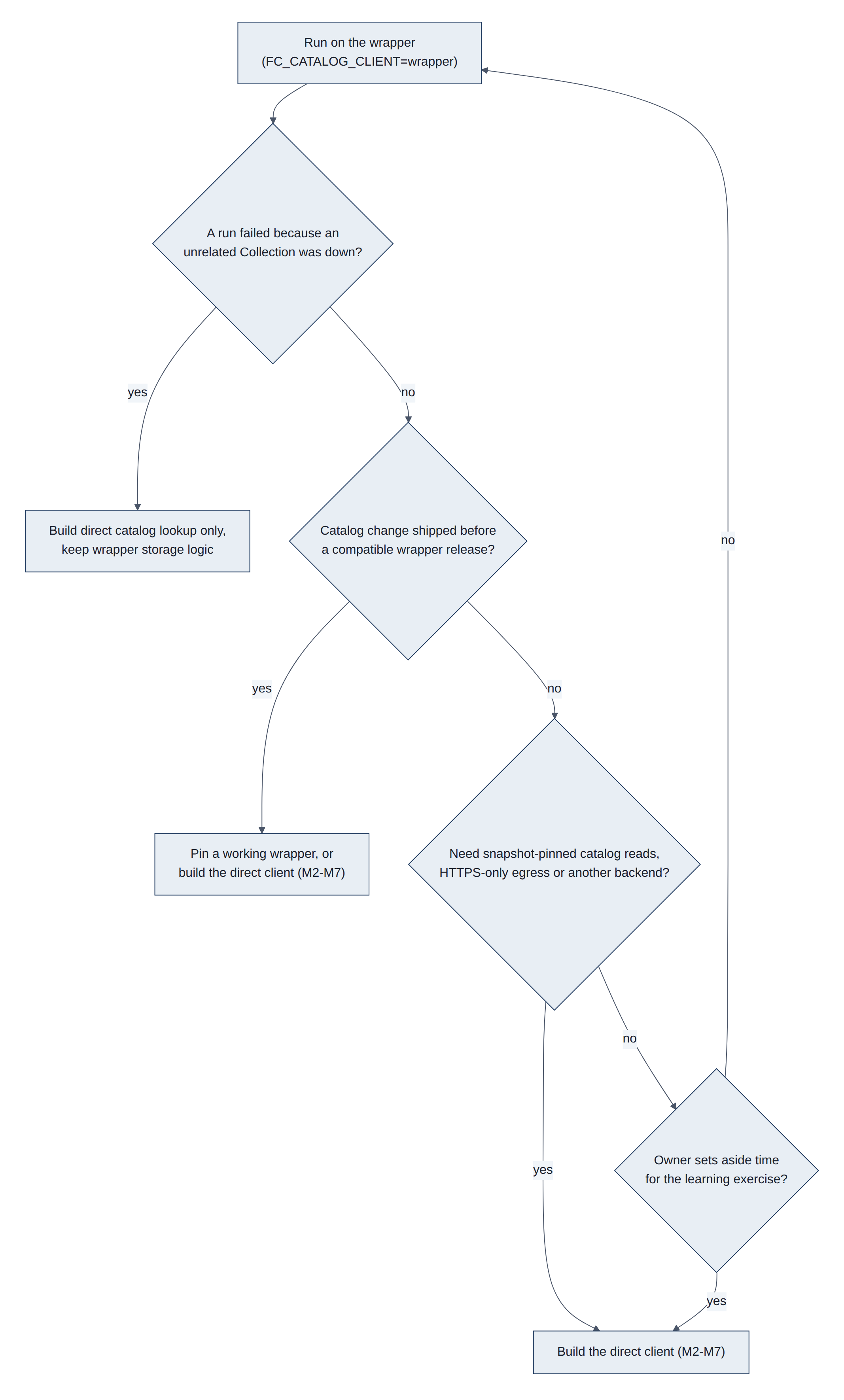
Run on the wrapper (FC_CATALOG_CLIENT=wrapper) until further notice. Triggers to revisit:
- Failure coupling bites: a run fails because an unrelated Collection was unreachable. Smallest fix: a direct client for catalog lookup only, still using the wrapper's storage logic.
- Wrapper lag: a dynamical.org catalog change ships before a compatible wrapper release.
- Need beyond the wrapper: snapshot-pinned reads from the catalog, HTTPS-only egress, or a storage backend choice the wrapper does not expose.
- Phase 3 virtual datasets: if lower latency matters for forecasts, decide whether to read
-virtualstores (wrapper already supports them) before writing any direct client. - Learning time: the owner chooses to do the exercise; follow M1-M7 in
07.
Until then, keep the wrapper pinned exactly and read its changelog at each upgrade.
Acknowledgements
Model data: NOAA, republished by dynamical.org under the Creative Commons Attribution 4.0 (CC BY 4.0) licence. Daily maps and normals: PRISM Group, Oregon State University. Station data: the National Weather Service (KPWM), volunteers of the Citizen Weather Observer Program via the Gladstone Weather Network and NOAA MADIS, and the Ambient Weather Network (house station). Solar production model: PVGIS, European Commission Joint Research Centre.
References
- dynamical.org STAC catalog and Collections, fetched 2026-10-26: catalog.json, noaa-hrrr-analysis, noaa-gfs-forecast-virtual
dynamical-catalog1.0.1 source: PyPI, GitHub- Icechunk documentation (repositories, sessions, virtual chunk containers)
- Zarr v3 core specification and the sharding codec
- STAC specification and the datacube extension
- Apache Parquet file format
- Cloud Optimized GeoTIFF and GDAL virtual file systems (
/vsizip/) - GRIB2: WMO Manual on Codes, FM 92; gribberish GRIB2 codec
- NOAA traditional access: NOMADS, HRRR on the NOAA Open Data Dissemination program (AWS)
- Stations: NWS ASOS, ASOS temperature and dew point sensors, Citizen Weather Observer Program, NOAA MADIS, Gladstone Weather Network, Ambient Weather WS-2902 specifications, Davis Vantage Pro2; station offsets and drift measured on lamp 2026-10-27 from the
wxtables,fc_prism_dailyandfc_analysis_hourly - Models: HRRR, GFS, GEFS, PRISM, dynamical.org catalog, PVGIS
- Format background: Cloud-Native Geospatial Foundation guide, OGC COG standard, OGC GeoTIFF standard, Icechunk specification, NCEP GRIB2 documentation, Parquet encodings, NetCDF, HDF5, MDN: HTTP range requests
- This project's measurements:
08-phase0-results.mdand this document (lamp, 2026-10-26), including the Zarr metadata, Parquet footer, Icechunk folder counts and PRISM GeoTIFF profile quoted in section 3
Appendix A. Sketch of catalog_direct.py
Not implemented. A starting point when the time comes, matching catalog.py's interface (Listing 2):
Listing 2. Sketch of catalog_direct.py, a direct catalog client.
"""Catalog client on plain HTTP + icechunk (D7 target)."""

import json
import time
import urllib.error
import urllib.request

import icechunk
import xarray as xr

from forecasting import settings
from forecasting.catalog import OpenedDataset

CATALOG = "https://stac.dynamical.org/catalog.json"
ALLOWED_SCHEMES = ("s3://", "https://")
_collections: dict[str, dict] = {}

def _get_json(url: str) -> dict:
    ua = "weather-forecasting/0.1"
    if email := settings.identify_email():
        ua += f" ({email})"
    for attempt in range(3):
        try:
            req = urllib.request.Request(url, headers={"User-Agent": ua})
            with urllib.request.urlopen(req, timeout=10) as resp:
                return json.load(resp)
        except urllib.error.HTTPError as e:
            if e.code not in (409, 429) or attempt == 2:
                raise
        except (urllib.error.URLError, TimeoutError):
            if attempt == 2:
                raise
        time.sleep(1.0)
    raise RuntimeError("unreachable")

def _collection(dataset_id: str) -> dict:
    if dataset_id not in _collections:
        links = _get_json(CATALOG)["links"]
        href = next(l["href"] for l in links if l["rel"] == "child"
                    and l["href"].rstrip("/").endswith(f"/{dataset_id}/collection.json"))
        coll = _get_json(href)
        if coll.get("id") != dataset_id or "icechunk" not in coll.get("assets", {}):
            raise ValueError(f"Unexpected collection for {dataset_id}")
        _collections[dataset_id] = coll
    return _collections[dataset_id]

def _storage(asset: dict) -> icechunk.Storage:
    href = asset["href"]
    if not href.startswith(ALLOWED_SCHEMES):
        raise ValueError(f"Unsupported storage scheme: {href}")
    if href.startswith("https://"):
        return icechunk.http_storage(base_url=href.rstrip("/"))
    bucket, prefix = href[len("s3://"):].split("/", 1)
    region = asset["xarray:storage_options"]["client_kwargs"]["region_name"]
    return icechunk.s3_storage(bucket=bucket, prefix=prefix.rstrip("/"), region=region,
                               anonymous=True)

def get_repository(dataset_id: str) -> icechunk.Repository:
    asset = _collection(dataset_id)["assets"]["icechunk"]  # by key, never by search
    containers = asset.get("icechunk:virtual_chunk_containers") or []
    if any(not c.get("credentials", {}).get("anonymous") for c in containers):
        raise ValueError("Virtual containers must be anonymous")
    authorize = icechunk.containers_credentials(
        {c["url_prefix"]: icechunk.s3_anonymous_credentials() for c in containers}
    ) if containers else None
    return icechunk.Repository.open(_storage(asset), authorize_virtual_chunk_access=authorize)

def open_dataset(dataset_id: str) -> OpenedDataset:
    session = get_repository(dataset_id).readonly_session("main")
    ds = xr.open_zarr(session.store, chunks=None, consolidated=False)
    return OpenedDataset(dataset_id, ds, session.snapshot_id, "direct")

def current_snapshot_id(dataset_id: str) -> str:
    return get_repository(dataset_id).lookup_branch("main")

def list_datasets() -> list[str]:
    links = _get_json(CATALOG)["links"]
    return sorted(l["href"].rstrip("/").split("/")[-2] for l in links if l["rel"] == "child")
Gaps to close before use: typed exceptions, offline tests with saved Collection JSON (valid, missing asset, bad scheme, credentialed container), and the M3 comparison.
Appendix B. Glossary
The first table spells out every acronym on this page. The second explains the other terms, in alphabetical order.
B.1 Acronyms
Table 23 spells out every acronym used in this report.
Table 23. Acronyms.
| Acronym | Stands for | What it is |
|---|---|---|
| .idx | Index file | NOAA's text sidecar listing where each message sits inside a GRIB2 file More |
| AIFS | Artificial Intelligence Forecasting System | ECMWF's machine-learning weather model More |
| API | Application Programming Interface | A web address a program calls to get data, such as ambientweather.net's More |
| ASOS | Automated Surface Observing System | The standard US airport weather station (KPWM) More |
| AWN | Ambient Weather Network | Ambient Weather's online service that receives the house station's readings More |
| AWS | Amazon Web Services | Amazon's cloud, home of S3 and of NOAA's open data More |
| B-tree | Balanced tree | A searchable index structure used inside databases and HDF5 files More |
| BIL | Band Interleaved by Line | A raw raster format PRISM used before COG More |
| blosc | (a name, not an acronym) | A fast compression wrapper that shuffles bytes before compressing; used in Zarr More |
| CC BY 4.0 | Creative Commons Attribution 4.0 | The licence of dynamical.org's data: free to use with credit More |
| CF | Climate and Forecast conventions | Shared rules for naming variables and units in NetCDF and Zarr More |
| CLI | Command-Line Interface | A program run by typing commands; here fc More |
| COG | Cloud Optimized GeoTIFF | A GeoTIFF laid out for partial reads over the web (3.8) More |
| CONUS | Contiguous United States | The lower 48 states, HRRR's coverage More |
| crc32c | Cyclic Redundancy Check, 32-bit, Castagnoli | A checksum that detects corrupted bytes, used in Zarr shard indexes More |
| cron | (from Chronos, Greek for time) | The Linux scheduler that runs lamp's jobs at set times More |
| CRS | Coordinate Reference System | The definition of how map coordinates relate to places on Earth More |
| CSV | Comma-Separated Values | Plain-text table, one row per line More |
| CWOP | Citizen Weather Observer Program | Network of volunteer stations that share data with NOAA More |
| D1 to D14 | Decisions 1 to 14 | This project's numbered design decisions; D7 is the open one on the wrapper More |
| DB | Database | An organised store of records, here MariaDB More |
| degC | degrees Celsius | Temperature unit used inside the model data More |
| degF | degrees Fahrenheit | Temperature unit used on the site More |
| E1248, E4229, E4279, G5290, G5544, G5907 | CWOP station IDs | Call signs assigned to volunteer stations (section 2.1) More |
| ECMWF | European Centre for Medium-Range Weather Forecasts | Europe's main forecasting centre More |
| EMC | Environmental Modeling Center | The NCEP centre that develops GFS and GEFS More |
| EPSG | European Petroleum Survey Group | Keeper of the numbered list of coordinate systems (EPSG:4269 is NAD83) More |
| FAA | Federal Aviation Administration | Co-operates the airport ASOS stations More |
| float32, float64 | 32-bit and 64-bit floating-point numbers | How computers store decimal numbers, with about 7 or 16 significant digits More |
| FM 92 | WMO code form 92 | The WMO's formal name for the GRIB2 format More |
| FTP | File Transfer Protocol | An older way to download files from a server More |
| GB, MB, KB | gigabyte, megabyte, kilobyte | About a billion, a million and a thousand bytes More |
| GCS | Google Cloud Storage | Google's object storage, the counterpart of S3 More |
| GDAL | Geospatial Data Abstraction Library | The standard open-source library for raster and map files More |
| GEFS | Global Ensemble Forecast System | NOAA's 31-member ensemble model (section 2.2) More |
| GET | HTTP GET request | The basic web request that fetches a resource More |
| GFS | Global Forecast System | NOAA's main global forecast model (section 2.2) More |
| GHI | Global Horizontal Irradiance | Sunlight power on a flat surface, in W/m2 More |
| GNU | "GNU's Not Unix" (a recursive name) | A free-software project whose tools include gzip More |
| GRIB2 | GRIdded Binary, edition 2 | WMO file format for model output (3.6) More |
| GYX | NWS Gray, Maine | Code of the local National Weather Service office More |
| gzip | GNU zip | A common lossless compression format More |
| HDD | Heating Degree Day | How far a day's mean temperature falls below 65 degF; drives heating use More |
| HDF5 | Hierarchical Data Format, version 5 | A traditional single-file scientific data format More |
| HRRR | High-Resolution Rapid Refresh | NOAA's hourly 3 km model (section 2.2) More |
| HTML | HyperText Markup Language | The language of web pages More |
| HTTP, HTTPS | HyperText Transfer Protocol (Secure) | How browsers and programs fetch web content More |
| ICAO | International Civil Aviation Organization | UN agency that assigns four-letter airport codes such as KPWM More |
| ID | Identifier | A unique name or number, such as a snapshot ID More |
| IFD | Image File Directory | The table of contents inside a TIFF (3.8) More |
| IFS | Integrated Forecasting System | ECMWF's physics-based model More |
| int64 | 64-bit integer | A whole number stored in 8 bytes More |
| ISO | International Organization for Standardization | Publisher of standards such as ISO 19115 for metadata More |
| JPEG 2000 | Joint Photographic Experts Group, 2000 standard | An image compression method GRIB2 can use for packing More |
| JSON | JavaScript Object Notation | Plain-text format for structured data More |
| JSONL | JSON Lines | A text file with one JSON record per line; lamp's run log uses it More |
| KPWM | ICAO airport code for Portland International Jetport | K (US) + PWM; also its table name More |
| kWh | kilowatt-hour | Unit of electrical energy on the electric bill More |
| L1, L2, L3 | Layers 1, 2 and 3 | This project's storage layers: grid cube, point tables, SQL views (3.4, 3.7) More |
| LZW | Lempel-Ziv-Welch | A lossless compression method used inside TIFF files More |
| M1 to M7 | Migration steps 1 to 7 | The steps for switching off the wrapper, in 07-client-migration.md More |
| MADIS | Meteorological Assimilation Data Ingest System | NOAA service that collects and quality-checks non-federal stations More |
| MAE | Mean Absolute Error | Average size of forecast errors, ignoring sign More |
| MDN | Mozilla Developer Network | Reference documentation for web standards More |
| METAR | Meteorological Aerodrome Report | The hourly airport weather report format More |
| MiB, GiB | mebibyte, gibibyte | 1,048,576 and 1,073,741,824 bytes (powers of two), slightly more than MB and GB More |
| MJ/m2 | megajoules per square metre | Daily sunlight energy on a surface; 1 MJ/m2 = 0.278 kWh/m2 More |
| ms | millisecond | One thousandth of a second More |
| NAD83 | North American Datum of 1983 | The coordinate system PRISM grids use More |
| NCEI | National Centers for Environmental Information | NOAA's long-term data archive More |
| NCEP | National Centers for Environmental Prediction | NOAA's centre that runs the operational models More |
| NetCDF | Network Common Data Form | A traditional scientific array file format More |
| NOAA | National Oceanic and Atmospheric Administration | The US agency for weather, oceans and climate More |
| NODD | NOAA Open Data Dissemination | NOAA's program that puts its data on public clouds More |
| NOMADS | NOAA Operational Model Archive and Distribution System | NOAA's traditional model download server More |
| NWS | National Weather Service | NOAA's forecasting arm More |
| OGC | Open Geospatial Consortium | Standards body for map data formats (COG, GeoTIFF) More |
| OPeNDAP | Open-source Project for a Network Data Access Protocol | A server protocol for subsetting remote scientific files More |
| p10, p50, p90 | 10th, 50th and 90th percentiles | Values with 10%, 50% and 90% of outcomes below them; p10 to p90 is an "8 in 10" range More |
| PAR1 | (Parquet's marker, not an acronym) | The four bytes that start and end every Parquet file More |
| PNG | Portable Network Graphics | Lossless image format used for the charts and diagrams More |
| PRISM | Parameter-elevation Regressions on Independent Slopes Model | Oregon State University daily weather maps (section 2.2) More |
| PROJ | (a name, not an acronym) | The standard library for converting between map projections More |
| PV | Photovoltaic | Solar electric panels More |
| PVGIS | Photovoltaic Geographical Information System | European Commission solar production model More |
| PWS | Personal Weather Station | A privately owned station such as ZASTMET More |
| QC | Quality Control | Checks that catch bad readings More |
| RAP | Rapid Refresh | NOAA's 13 km hourly model that HRRR is nested in More |
| README | "read me" | The overview file of a code folder More |
| RFC | Request for Comments | The numbered internet standards series (CSV is RFC 4180) More |
| RMSE | Root Mean Square Error | Like MAE but weighs large errors more More |
| S3 | Simple Storage Service | Amazon's object storage, where dynamical.org's data lives More |
| SQL | Structured Query Language | The language for asking questions of tables More |
| STAC | SpatioTemporal Asset Catalog | A JSON standard for listing geospatial datasets (3.3) More |
| THREDDS | Thematic Real-time Environmental Distributed Data Services | A traditional catalog and data server for scientific files More |
| Thrift | Apache Thrift (a name, not an acronym) | A compact binary encoding Parquet uses for its footer More |
| TIFF | Tagged Image File Format | A long-standing image file format More |
| TMP | Temperature | GRIB2's short name for temperature, as seen in .idx files More |
| U1 to U13 | Use cases 1 to 13 | The questions this project answers, listed in 02-use-cases.md More |
| URL | Uniform Resource Locator | A web address More |
| US | United States | More |
| UTC | Coordinated Universal Time | The world reference clock; Maine is UTC-5 in winter, UTC-4 in summer More |
| UV | Ultraviolet | Part of sunlight, measured by the house station More |
| W/m2 | watts per square metre | Unit of sunlight power More |
| WMO | World Meteorological Organization | UN agency that sets weather data standards such as GRIB2 More |
| WS-2902 | Ambient Weather model number | The house station's model; WS stands for weather station (the stations table lists a WS-2000) More |
| XML | Extensible Markup Language | Text format for structured data, older than JSON More |
| ZASTMET | The house station's name | The owner's name for the station at the house; also its table name More |
| zstd | Zstandard | A modern lossless compression method, used in Zarr and Parquet More |
B.2 Terms
Table 24 explains the other terms, in alphabetical order.
Table 24. Terms.
| Term | Meaning |
|---|---|
| Analysis | A model's best estimate of the weather at a past moment, blending a short forecast with observations (2.2.1) More |
| Array | A grid of numbers with several dimensions, such as time, north-south and east-west More |
| Aspirated shield | A thermometer housing with a fan that pulls outside air past the sensor, so sunshine cannot warm it More |
| Balance point | The daily mean temperature below which heating (or above which cooling) starts to use energy (4.3.5) More |
| Baseline | A simple forecast to beat: persistence or climatology More |
| Bias | The average error, with sign: a positive bias means the forecast or station runs warm More |
| Billing period | The days between two gas meter reads; a bill covers one, usually about 30 days More |
| Branch | A named pointer to the newest snapshot of a repository (Icechunk, Git) More |
| Byte range request | Asking a web server for only part of a file, such as bytes 5,000 to 9,000 More |
| Calibration | Adjusting forecast ranges using past errors so that "8 in 10" really happens 8 times in 10 More |
| Change-point model | A usage model that is flat between two balance points and rises in a straight line beyond each (4.3.5) More |
| Chunk | One separately stored and compressed block of a larger array More |
| Climatology | The normal weather for a date, averaged over 1991-2020; a baseline forecast More |
| Cloud-native | Stored so that programs can read just the piece they need directly from object storage More |
| Codec | One encoding or compression step applied to stored bytes, reversed when reading More |
| Cold air pooling | Cold, dense air settling in low spots on calm, clear nights, so valleys read colder More |
| Column store | A table format that keeps each column together (Parquet), the opposite of a row store More |
| Commit | Saving one set of changes as a new snapshot More |
| Compression | Encoding data in fewer bytes; lossless keeps every bit, lossy rounds slightly More |
| Coverage | How often the observed value fell inside a forecast range; the target for p10 to p90 is 80% More |
| Data assimilation | Combining observations with a model's short forecast to estimate the current weather More |
| Dimension | One direction of an array, such as time or latitude More |
| Drift | A slow change in a sensor's readings over months, from aging, dirt or a change in siting More |
| DuckDB | An in-process SQL database that queries Parquet files and other databases directly More |
| dynamical.org | A non-profit that republishes NOAA and ECMWF model data in cloud-native formats More |
| Ensemble | A set of forecasts from slightly different starting points; their spread shows uncertainty More |
| Fill value | The value an array reports for missing data or for chunks never written (often NaN) More |
| Footer | Metadata stored at the end of a file, as in Parquet More |
| Forecast | A model run projecting the weather forward from its run time More |
| Grid cell, grid square | One box of a model's grid; its value is an average over the box More |
| Ground truth | Observations treated as what really happened, used to score forecasts More |
| Hive partitioning | Folder names of the form key=value (such as year=2026) that act as table columns More |
| Icechunk | A transactional, versioned storage engine for Zarr data (3.4) More |
| Initialization time, run time | The moment a forecast run starts from More |
| Known-weather floor | The error left when a usage model is fed the weather that actually happened; no forecast can do better (4.3.1) More |
| Lambert conformal projection | A cone-shaped way of flattening the Earth, used by HRRR's grid More |
| lamp | The small Linux server at the house that runs this project More |
| Lead time | How far ahead of its run time a forecast is, such as "24 hours ahead" More |
| Manifest | Icechunk's list of where every chunk is stored More |
| MariaDB | The relational database holding the station readings and household records More |
| Member | One of the runs in an ensemble More |
| Metadata | Data about the data: shape, units, chunk layout, where things are stored More |
| Model (weather model) | A computer simulation that steps the atmosphere's physics forward on a grid More |
| NaN | "Not a Number", the standard marker for a missing floating-point value More |
| Net grid use | Household use minus solar production: drawn from the grid when positive, sent to it when negative More |
| Normals | Average weather for each calendar day over a 30-year period (here 1991-2020) More |
| Object storage | Internet-scale file storage (such as S3) where every file has a web address More |
| Offset | The steady difference between a station and a reference; a change in it signals a problem More |
| Out of sample | Scored on data that was not used to fit the model, so the score is honest More |
| Overview | A reduced-resolution copy of a raster for zoomed-out views More |
| Parquet | A columnar file format for tables (3.7) More |
| Passive radiation shield | A stack of white plates that shades a thermometer without a fan More |
| Persistence | The baseline forecast "the future will be like the latest observation" More |
| Pyranometer | A sensor for sunlight power; ZASTMET's is a light (lux) sensor converted to W/m2 More |
| Raster | A grid of pixels, each holding a value More |
| Reanalysis | A consistent analysis of past decades rerun with one modern model More |
| Recent level | How far above or below the model household use has run over the past four weeks, added to each forecast (4.3.5) More |
| Repository | A store with version history (Icechunk, Git) More |
| Row group | A block of rows inside a Parquet file, stored column by column More |
| Shard | A bundle of chunks stored as one object, with an index of where each chunk sits More |
| Skill score | 1 minus a forecast's error divided by a baseline's error: 1 is perfect, 0 no better than the baseline More |
| Snapshot | The complete, frozen state of a repository after one commit, with its own ID More |
| Snapshot isolation | Every read sees one whole snapshot, never a half-finished update More |
| Solar day | 06:00 UTC to 06:00 UTC, the window used to total a day's forecast sunlight (4.3.3) More |
| Tag | A permanent name for one snapshot More |
| Therm | A unit of gas energy on the gas bill, 100,000 British thermal units, or about 29.3 kWh More |
| Tile | A square block of pixels stored on its own in a raster More |
| Usage model | The calculation that turns weather into kWh produced or therms used, fitted on past records More |
| Valid time | The moment a forecast value describes (run time plus lead time) More |
| Virtual dataset | A store that points to data inside other files instead of copying it More |
| Wrapper | dynamical.org's helper library dynamical-catalog, which finds and opens their datasets More |
| Zarr | A format for chunked, compressed arrays stored as many objects (3.5) More |