← Back to the main page (temperature charts, energy costs, and residential solar).

Forecasts and Model Checks — Cumberland Center, Maine

Dated analysis: Forecast performance: results as of 27 October 2026 (PDF) explains what this page showed that day, with each result put in context.

Forecasts and how accurate they have been

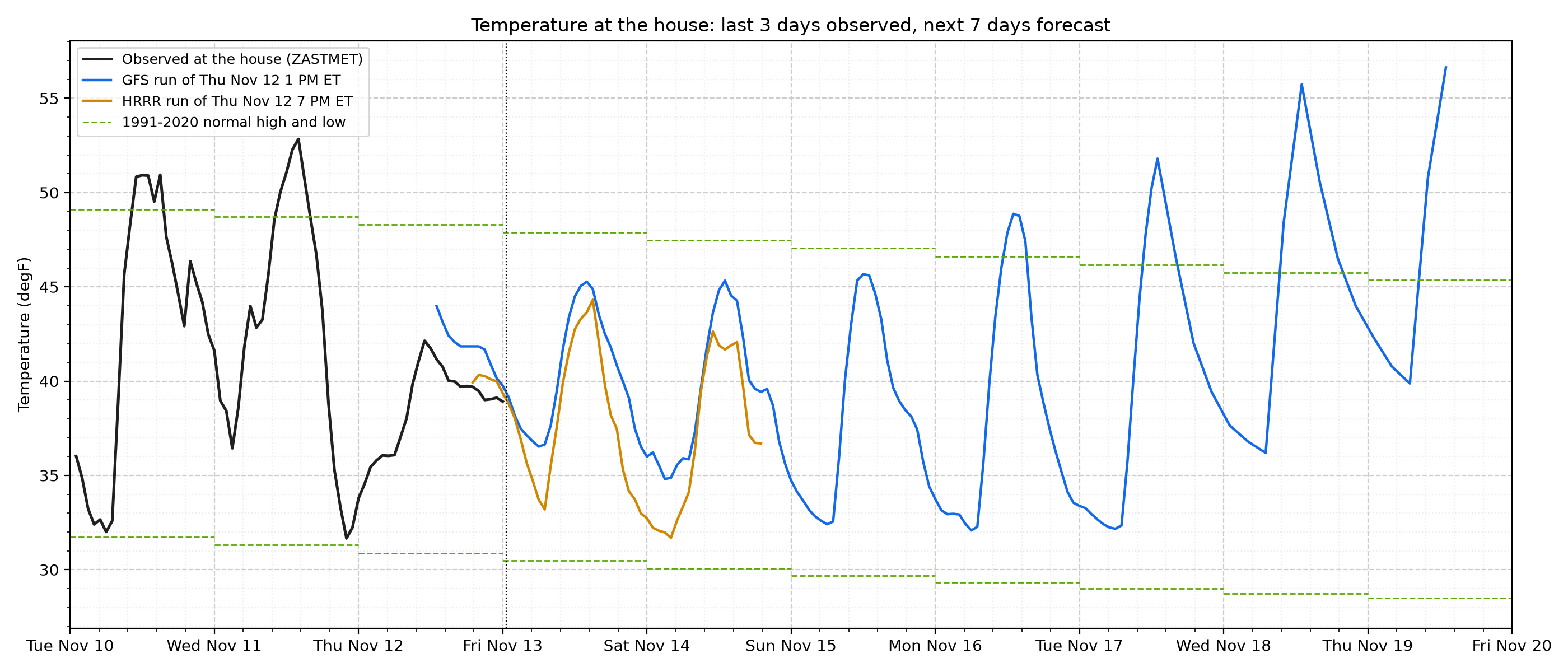
Figure 1. Temperature Outlook at the House - The black line is the house station over the last three days; the colored lines are the newest runs of two NOAA models. HRRR is a 3 km model that runs every hour; its four daily runs that reach 48 hours ahead are kept here. GFS is the global model, run four times a day out to 16 days (7 shown). Dashed green lines are the 1991-2020 normal high and low from PRISM. Times are Eastern. The accuracy of these models over recent months is in the next two figures, so read the forecast with its track record.

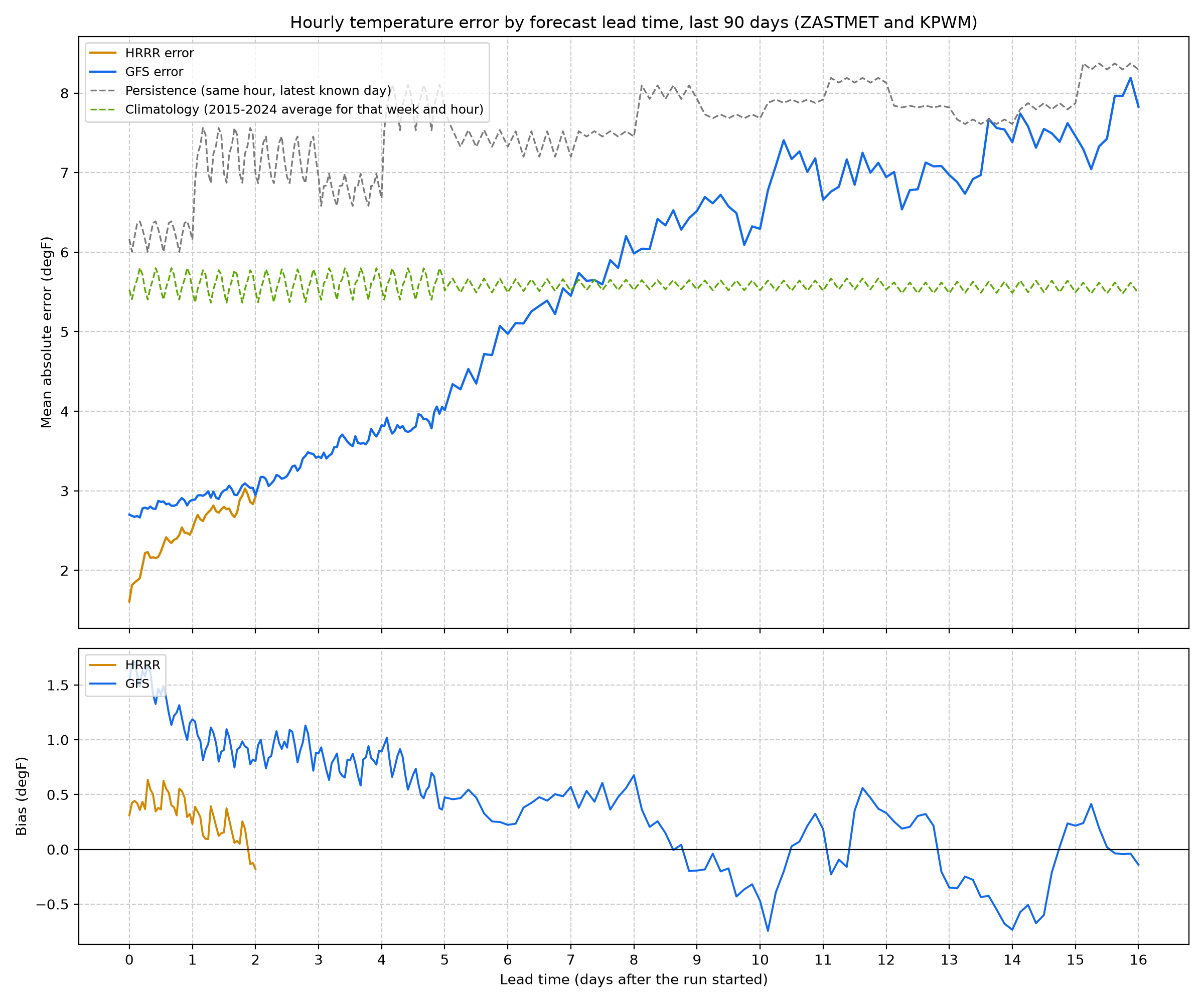
Figure 2. Hourly Forecast Error by Lead Time - Each line is the average size of the temperature error (ignoring sign) for all runs in the last 90 days at the house and the airport, by how far ahead the forecast was. HRRR is off by about 2.0 degF in its first 6 hours and 2.8 degF on day 2; GFS by 3.0 degF on day 2 and 5.3 degF at one week. Two simple baselines show whether the models add value: persistence (tomorrow at this hour will be like today; 7.2 degF on day 2) and climatology (the usual temperature for that week and hour; 5.6 degF). The lower panel shows bias: above zero means the model ran warm.

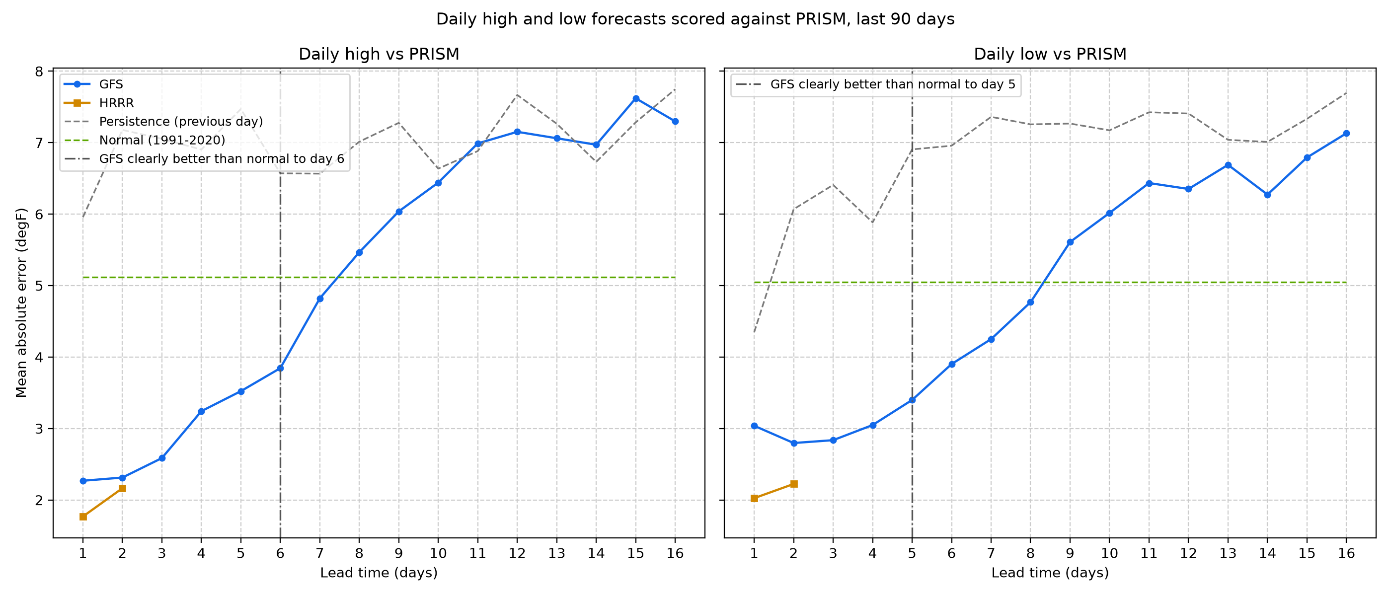
Figure 3. Daily High and Low Skill - Forecast daily highs and lows scored against PRISM's observed values for the same day (which do not use the house station), against the 1991-2020 normal and against the previous day's observed value. GFS one-day-ahead highs are off by 2.3 degF on average, against 5.1 degF for the normal. GFS is clearly better than the normal through day 6 for highs and day 5 for lows (dash-dot lines): there the lower end of the 95% interval of its skill, from a bootstrap that resamples whole weeks, is above zero. On average it stays ahead through day 7 for highs and day 8 for lows, though past the dash-dot lines not by enough to be sure; beyond that, the normal is the better guess. HRRR covers days 1 and 2 only.

Scored runs stored: GFS 430, HRRR 430. Scores update as new runs and observations arrive; PRISM values are provisional for six months.

Heating outlook: the next two weeks

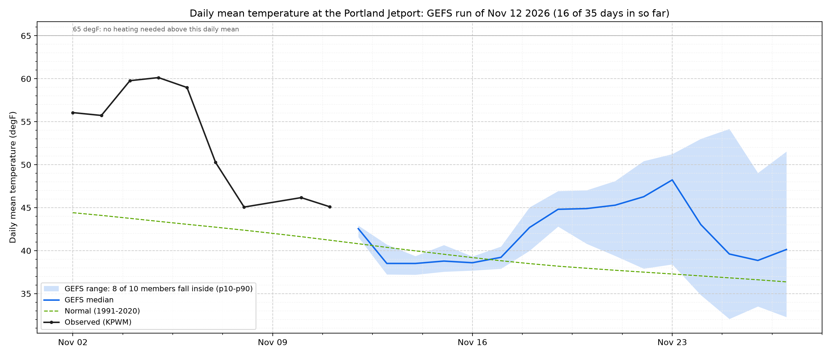
Figure 4. 35-Day Temperature Outlook - NOAA's global ensemble (GEFS) runs the same forecast model 31 times with slightly different starting conditions. Where the runs agree the band is narrow; where they spread out, the weather is less predictable. The blue band holds the middle 80% of the runs for each day's mean temperature, the blue line is the middle run, the dashed green line the 1991-2020 normal (adjusted to the station), and the black dots the last ten observed days. This band is the raw model output: in the first week it is too narrow (see Figure 6), so the cost outlook uses calibrated ranges instead. Beyond about two weeks the forecast is little better than the normal (Figure 6), which is why the cost outlook stops at 14 days. A run arrives over several hours, so the newest one may not reach 35 days yet.

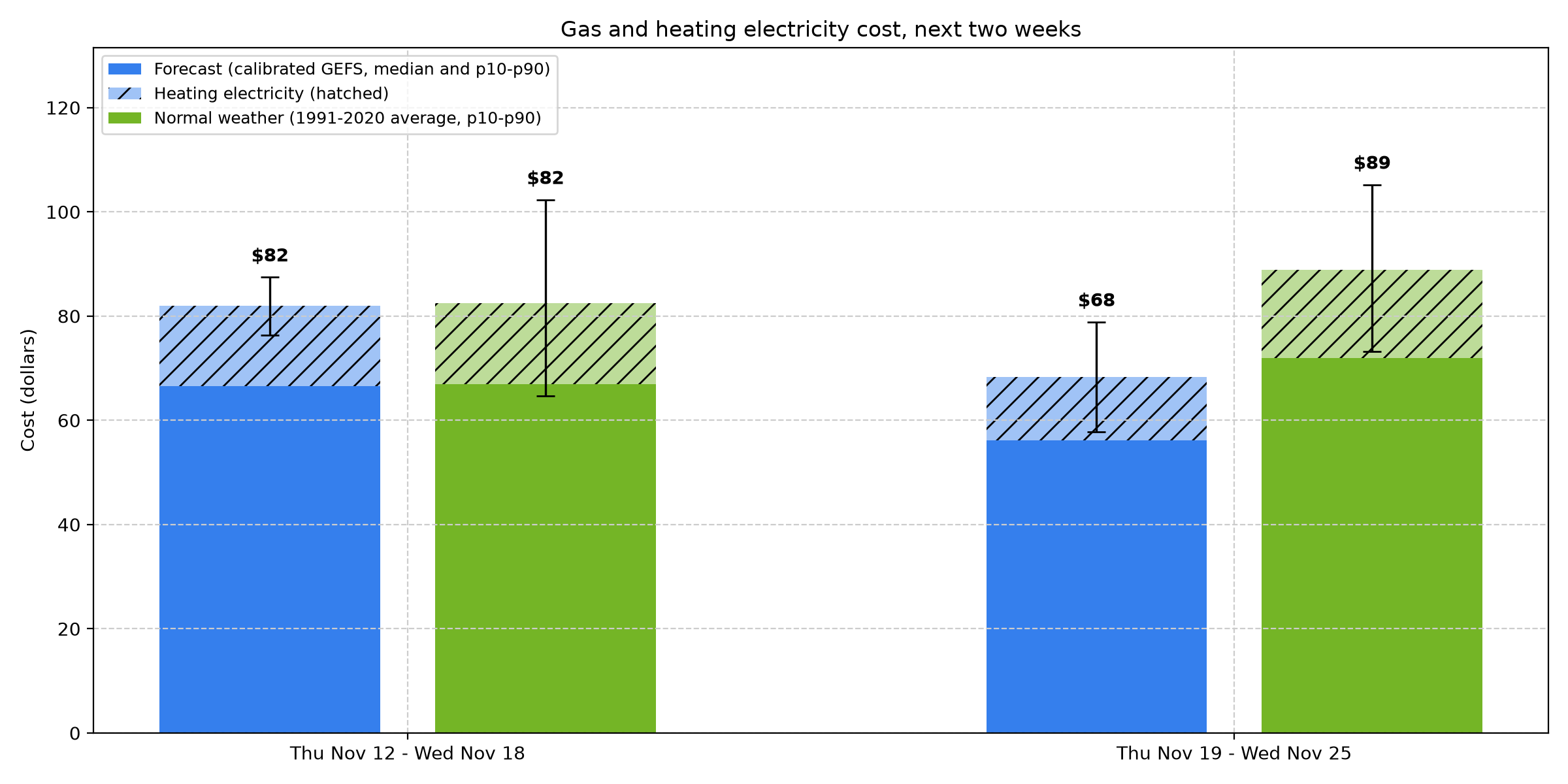
Figure 5. Heating Cost Outlook - What the next two weeks of gas and heating electricity should cost, from the forecast heating degree days (HDD: degrees the daily mean falls below 65 degF, summed over the days). The house heats with a gas boiler, so most of the cost is gas: about 0.15 therms per HDD plus 0.6 therms a day for hot water and cooking (fitted on 33 bills, r = 0.97). Electricity adds 0.33 kWh per HDD (circulator and blower). This week: $82 (8 in 10 chance between $76 and $87), against $82 in normal weather. Next week: $68 ($58 to $79), normal $89. The ranges are calibrated on past GEFS errors (Figure 6). Gas is priced at the latest bill's rate ($1.90 per therm with delivery, bill of 2026-09-03, plus $1.08 a day in fixed charges). Winter supply prices have been much higher (the March 2026 bill was over $3.80 per therm), so in winter read the dollars as a floor and the therms as the firmer number (31 therms this week). Electricity is priced at the standard tariff ($0.264/kWh), as on the main page, before any solar credit.

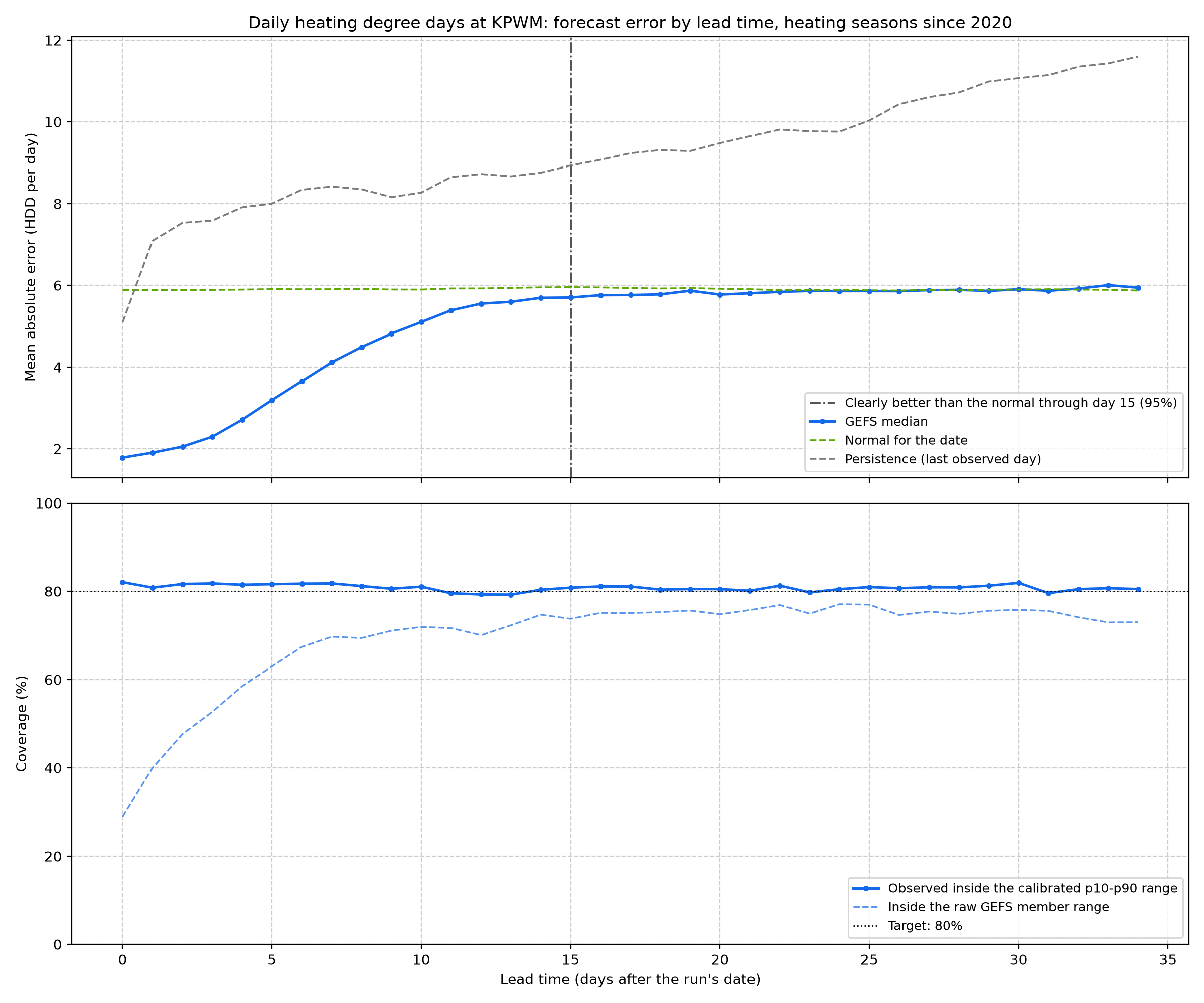
Figure 6. How Good the Outlook Has Been - Every daily GEFS run since October 2020 scored against the Portland Jetport's observed HDD in heating seasons (October-April). The middle of the forecast is clearly better than the normal for the date through day 15 (dash-dot line): there the lower end of the 95% interval of its skill, from a bootstrap that resamples whole weeks, is above zero. Its average stays slightly ahead through about day 27, but after day 15 the skill is at most 0.04, too small to tell apart from the normal. It beats persistence (every day repeats the last observed one) at every lead. The lower panel is the honesty check for the range, which should hold the observed value 8 times in 10. The raw members (dashed) are too confident early on: they held the observed week only 55% of the time, and missed mostly on the cold side. The calibrated range shifts the centre by the average past error and widens the spread in proportion to how much the members disagree; each season is scored with a calibration fitted on the other seasons only. It held the observed week 81% of the time (the next week 77%; at the house station 83%). It is still much narrower than the range of normal weather (33 HDD wide against 91). For one-week totals the forecast misses by 10 HDD on average, against 27 for the normal and 41 for persistence; that is about $4 of weekly heating cost at current prices. By season:

Heating season (Oct-Apr)	Weekly forecasts	GEFS error (HDD)	Normal error	Persistence error	Inside raw GEFS range	Inside calibrated range	Inside normal range
2020-21	204	11	25	43	53%	75%	81%
2021-22	212	9	24	43	67%	86%	87%
2022-23	212	11	34	42	49%	79%	74%
2023-24	146	9	27	37	57%	86%	75%
2024-25	212	11	24	42	50%	78%	79%
2025-26	192	10	27	39	51%	83%	81%
2026-27	33	8	19	34	58%	88%	85%

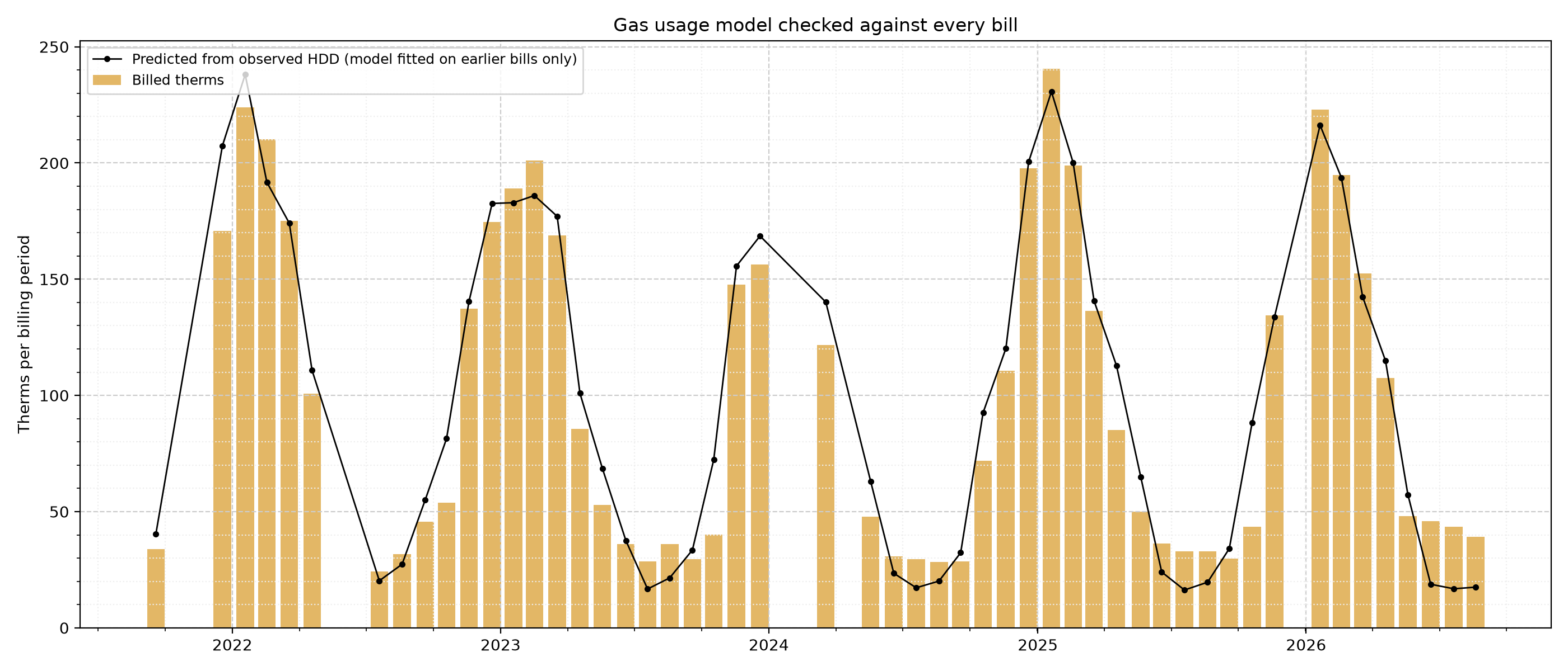
Figure 7. Gas Usage Model Against the Bills - Gas is metered only once a month, so the weekly cost cannot be checked directly. Instead each bill since late 2021 is predicted from the HDD that actually occurred, using a model fitted only on the bills before it. The model is off by 22% per bill on average (6% for November to March bills, when heating dominates). The outlook's range covers the weather, not this usage error, so the true range is a little wider.

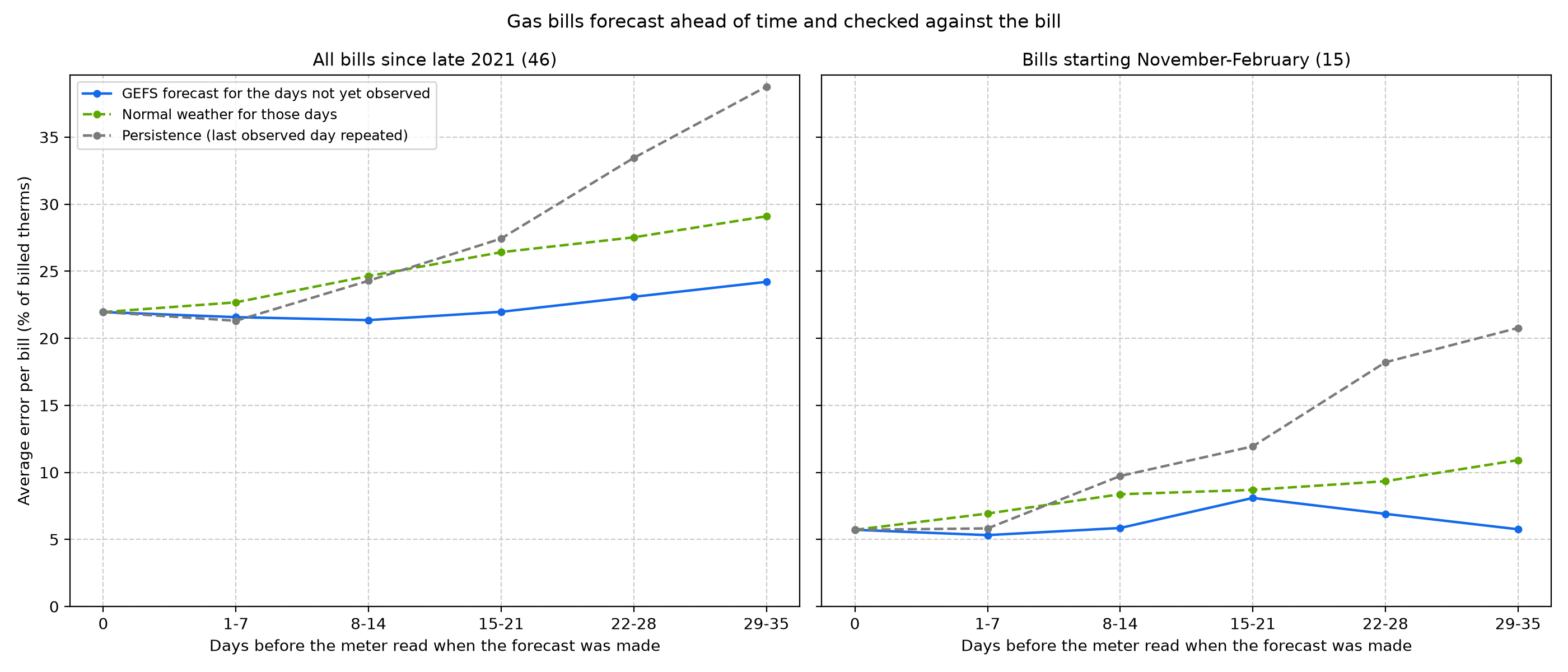
Figure 8. Gas Bills Forecast Ahead of Time - The previous figure checks the usage model with the weather already known. This one checks the whole chain, weather forecast included, the way a forecast would really have been used. For each bill, every GEFS run from the 35 days before the meter read is replayed: days before the run use the observed HDD, the rest the run's calibrated forecast, and the usage model (fitted on earlier bills only) turns the total into therms. The same days are also filled with the normal and with persistence. At 0 days the weather is fully known, so that point is the usage model's own error (22% per bill over all 46 bills, 6% for the 15 winter bills). Forecast 29 to 35 days ahead, when almost every day of the bill is still in the future, the error is 24% (6% in winter), against 29% (11%) for normal weather and 39% (21%) for persistence. In dollars at each bill's own rate: about $28 per bill against $37 for the normal. Most of a month-ahead bill error is the usage model, not the weather forecast. Winter has only 15 bills, so its points scatter by a few percent.

Solar: what the sky delivered and what the panels made

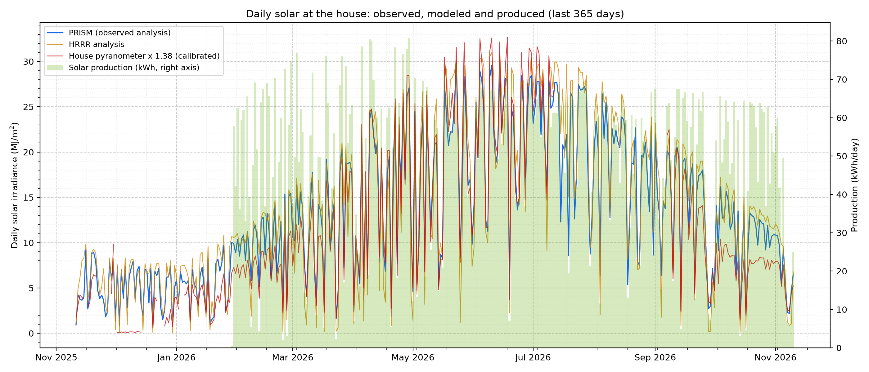
Figure 9. Daily Solar at the House - Daily solar energy reaching the house, from three sources, with the array's production. PRISM (Oregon State University) is an observation-based daily analysis; HRRR is NOAA's hourly 3 km model analysis, summed to days; the house pyranometer on the ZASTMET station is scaled by its calibration factor (1.38, Figure 10). All three use the PRISM day, which runs from 8 am to 8 am Eastern (12:00 UTC); nearly all of its sunlight falls on the previous calendar day, which is the production day shown.

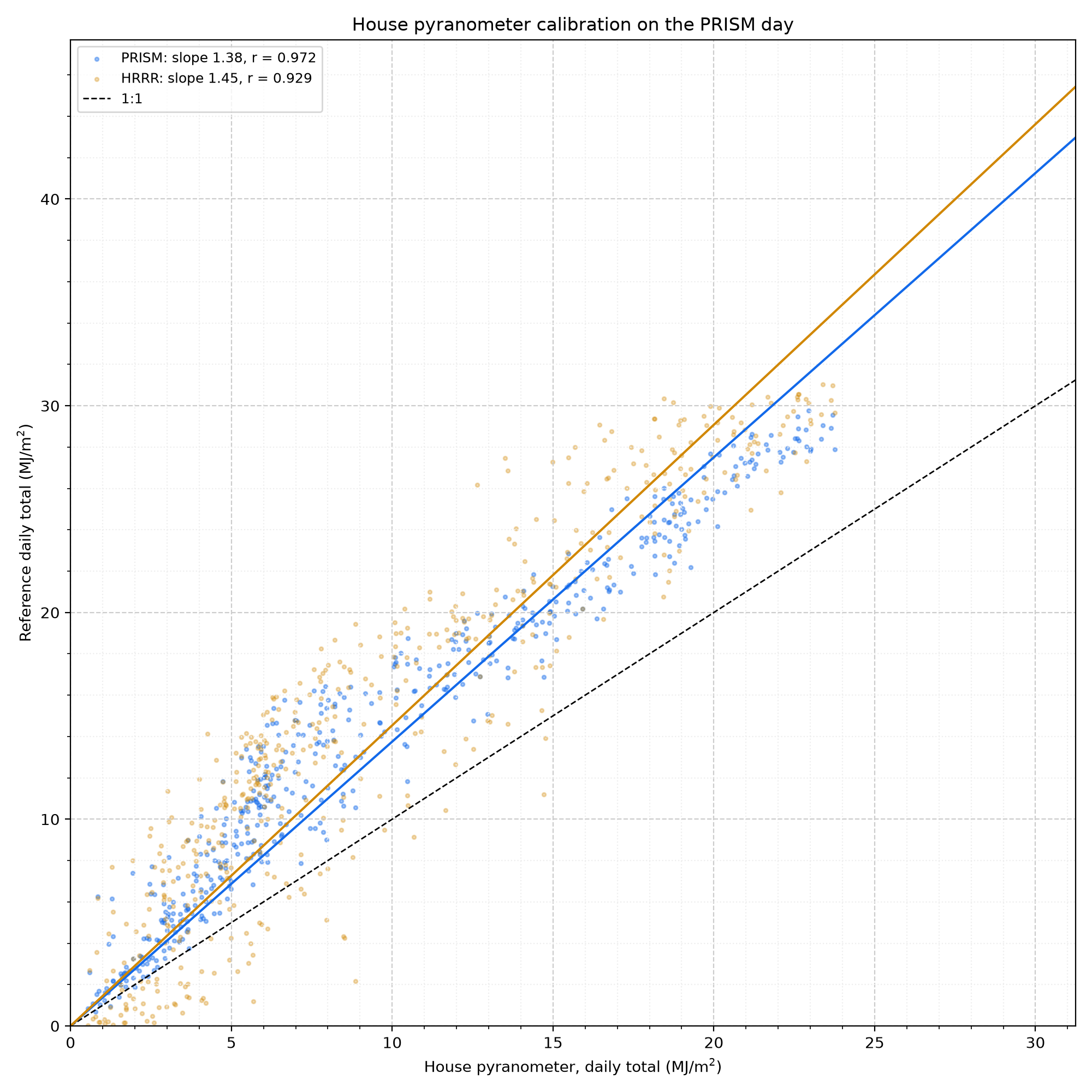
Figure 10. House Pyranometer Calibration - The house sensor tracks PRISM closely (r = 0.972) but reads low: PRISM is 1.38 times the house value on average over 500 complete days (Jan 2024 to Nov 2026). Against HRRR the factor is 1.45 (r = 0.929); HRRR runs 1.06 times PRISM, partly because it reports an instant at the top of each hour rather than an average. These factors are applied before the house readings are used as irradiance.

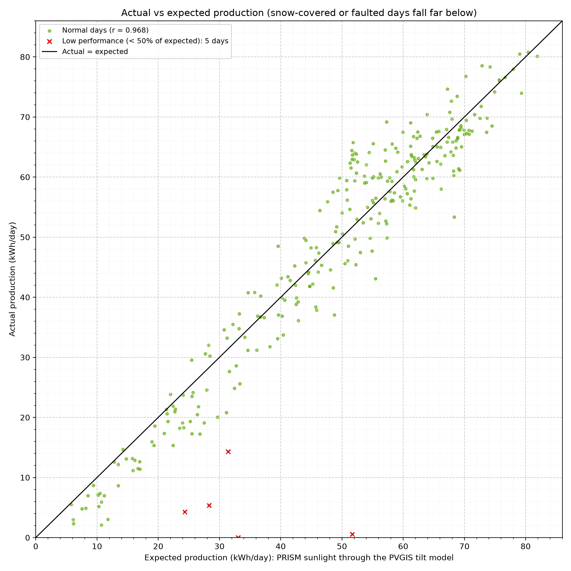
Figure 11. Actual vs Expected Production - Each point is one day since the system started. PRISM measures sunlight on flat ground; the panels are tilted 37° toward the southwest (215°), which catches far more of the low winter sun. The expected value converts each day's PRISM sunlight with the PVGIS model of this exact array, month by month, then scales it by how the real array compares: it delivers 101% of the unshaded PVGIS model (r = 0.968, typical daily error 8%, 282 days). That is in line with the model, so shade and other losses are about what PVGIS assumes (14%). 5 days made less than 50% of the expected amount despite real sun; in winter these are almost always snow on the panels.

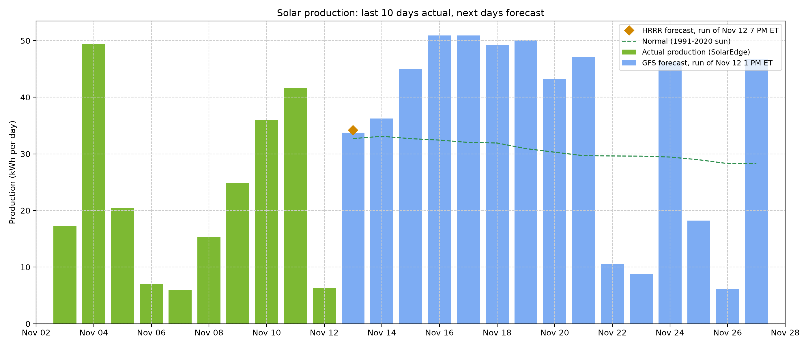
Figure 12. Solar Production Forecast - Expected production for today and the coming days, from the sunlight forecast by two NOAA models: GFS (Global Forecast System, bars, 16 days) and HRRR (High-Resolution Rapid Refresh, diamonds, today and tomorrow). Each day's forecast sunlight goes through the same production model as Figure 11. Each model forecasts a little more sunlight than PRISM measures (GFS 1.02 and HRRR 1.08 times), so its sunlight is scaled down by that ratio first. Tomorrow: GFS 34 kWh, HRRR 34 kWh. The dashed line is production in normal weather for the date. Snow on the panels is not forecast. The accuracy of these forecasts is in the next figure.

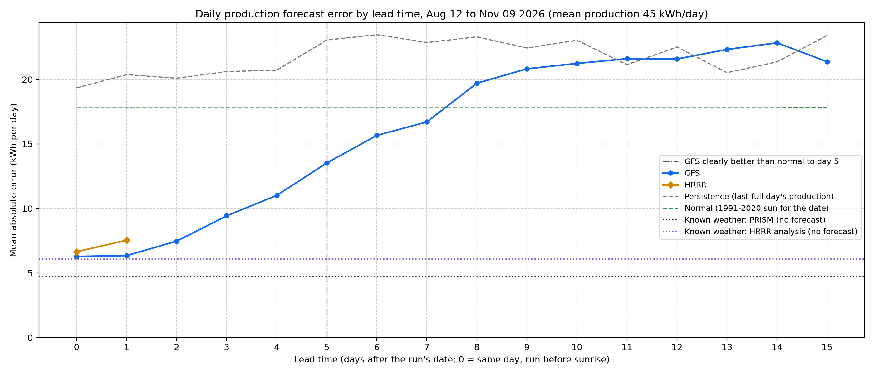
Figure 13. Solar Forecast Error by Lead Time - How far off the production forecasts were, on average, by how many days ahead they were made, over the last 90 days. A forecast for tomorrow missed by 6.3 kWh (GFS) and 7.5 kWh (HRRR), about 14% of a typical day's 45 kWh. Guessing the normal for the date misses by 17.8 kWh and repeating the last day by 20.4 kWh. At one week GFS misses by 16.7 kWh. GFS is clearly better than the normal through day 5 (dash-dot line): there the lower end of the 95% interval of its skill, from a bootstrap that resamples whole weeks, is above zero. On average it stays ahead through day 7, though after day 5 not by enough to be sure; after that, the normal is the better guess. The dotted lines are the floor: the same production model driven by the sunlight that actually arrived, with no forecast involved. Using PRISM's measured sunlight it misses by 4.8 kWh, and using the HRRR analysis (the model's own picture of what happened) by 6.1 kWh. The gap between a line and the floor is the part of the error that comes from forecasting the weather; the floor itself is the production model's own error (snow, shade, haze, and the step from flat-ground sunlight to tilted panels). Since the array started (287 days), the floors are 4.3 kWh (PRISM) and 7.4 kWh (HRRR analysis).

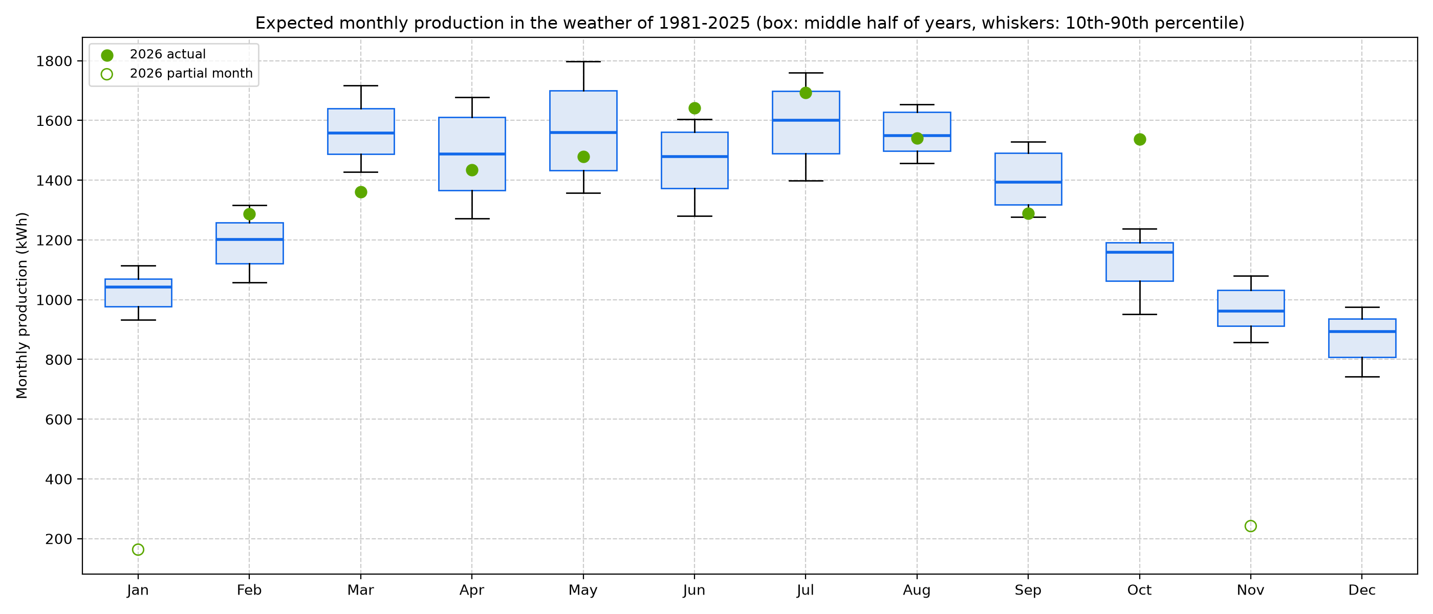
Figure 14. Expected Production in Past Weather - The model from Figure 11 applied to PRISM's daily sunlight for 1981-2025 shows what this array would have made in each past year's weather. A median year gives about 15,794 kWh; one year in ten falls below 15,413 kWh and one in ten exceeds 16,348 kWh. The sunniest year was 1999 (17,254 kWh) and the dullest 2023 (15,064 kWh). These figures leave out snow cover, which the model does not include. Dots show this year's actual months. PRISM advises against reading long-term trends from these series, so this shows spread, not trend.

Electricity: household use, solar and the grid

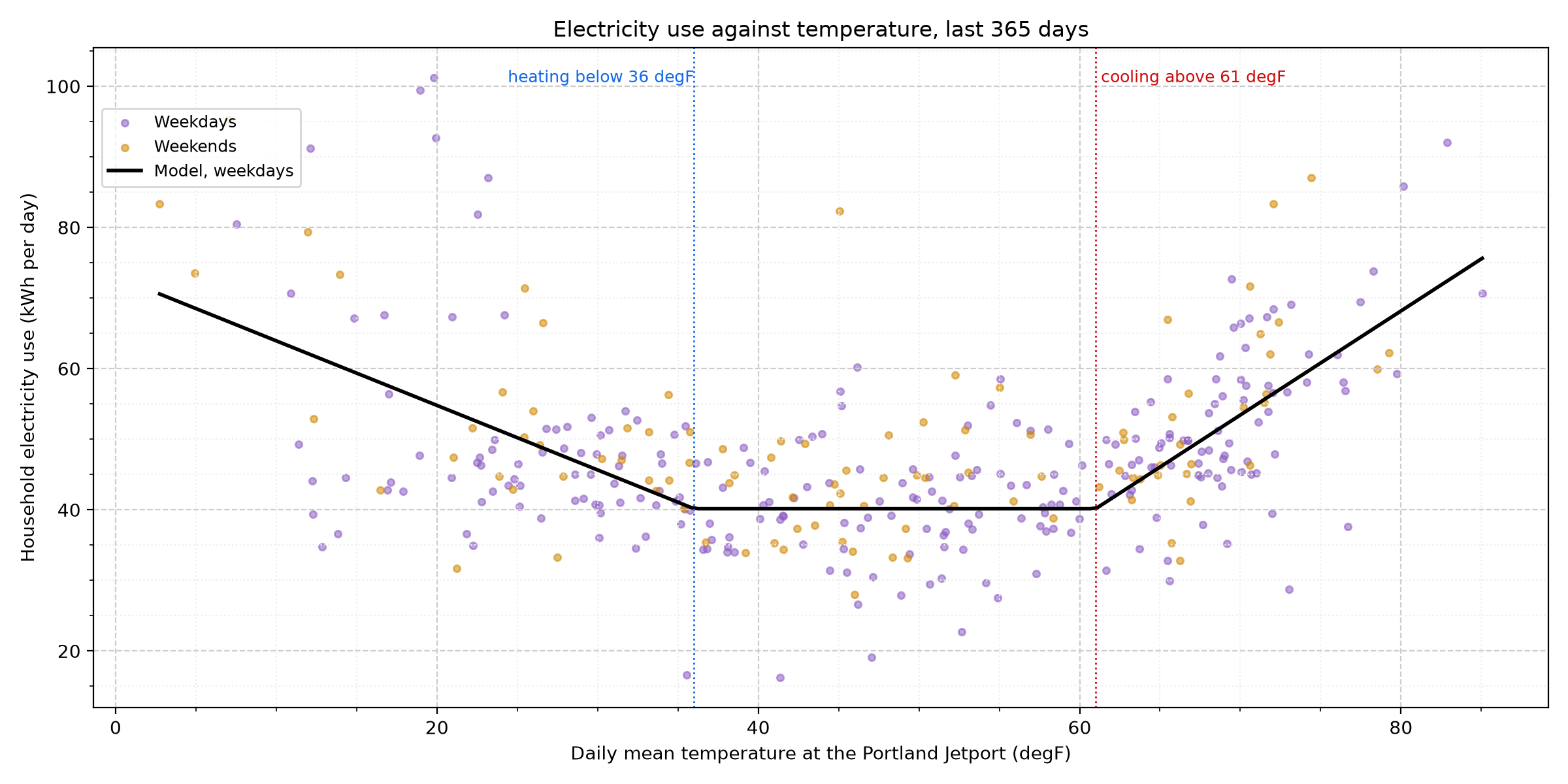
Figure 15. Electricity Use and Temperature - Each dot is one day's household electricity use (all appliances, whatever the source: grid or solar). Before the solar array the utility meter measured it directly; since then it is the meter's import plus solar production minus export, or SolarEdge's own monitoring where the meter data has not been loaded yet (scaled by 1.038 to match the meter). The line is a change-point model: a base of 40 kWh a day, plus 0.91 kWh for each degree the daily mean falls below 36 degF (electric loads that grow in the cold, such as the gas boiler's pumps and blower, lighting and longer evenings indoors) and 1.47 kWh for each degree above 61 degF (air conditioning), plus 3.3 kWh on weekends. Temperature explains only part of the day-to-day swing (r = 0.60; typical scatter 10 kWh a day): the rest is how the household lives, which no weather forecast can know. The model is refitted every month on the year before it.

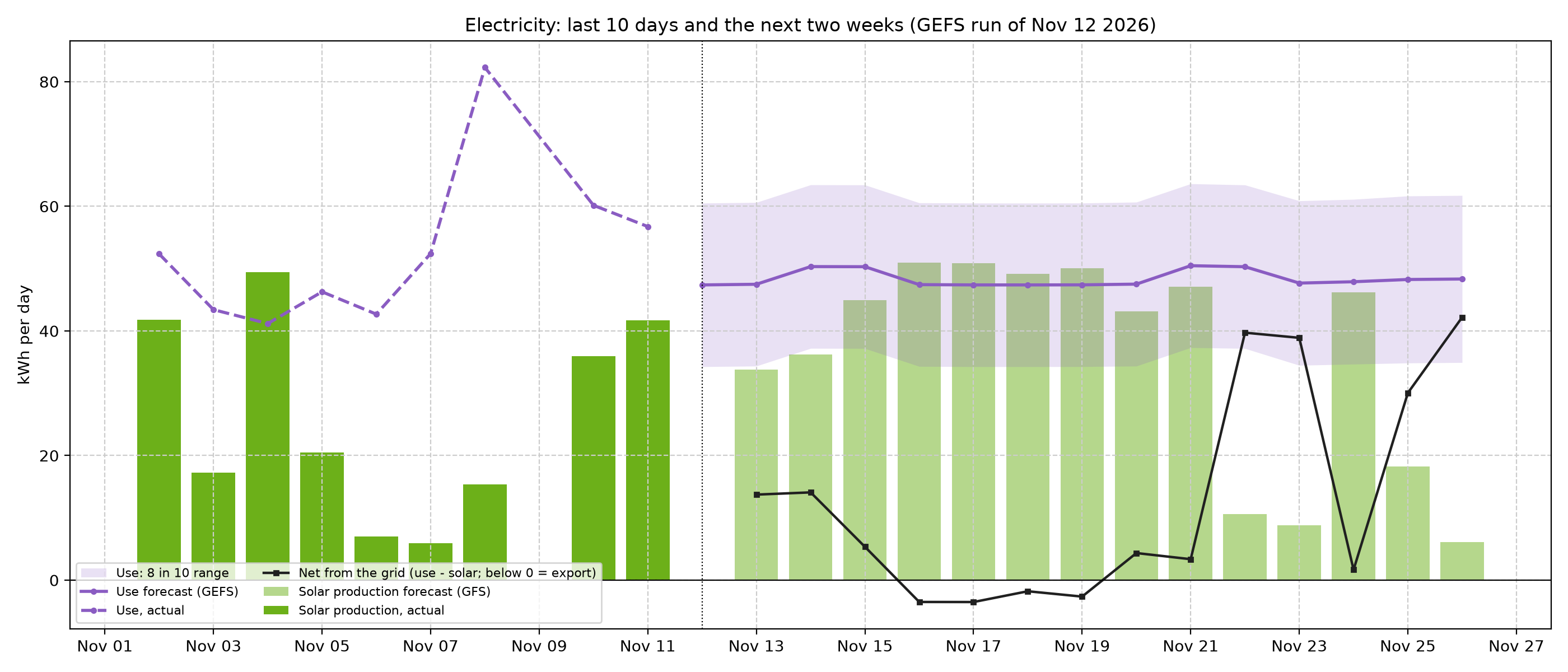
Figure 16. Electricity Outlook - Use for the next two weeks comes from each of the 31 GEFS temperature forecasts through the model, plus the household's recent level (how far above or below the model use has run over the last 28 days). The shaded band adds the model's own day-to-day scatter to the spread of the weather forecasts. Solar is the GFS forecast from Figure 12. Their difference is the net draw from the grid; below zero the house exports. This week: about 338 kWh of use and 266 kWh of solar.

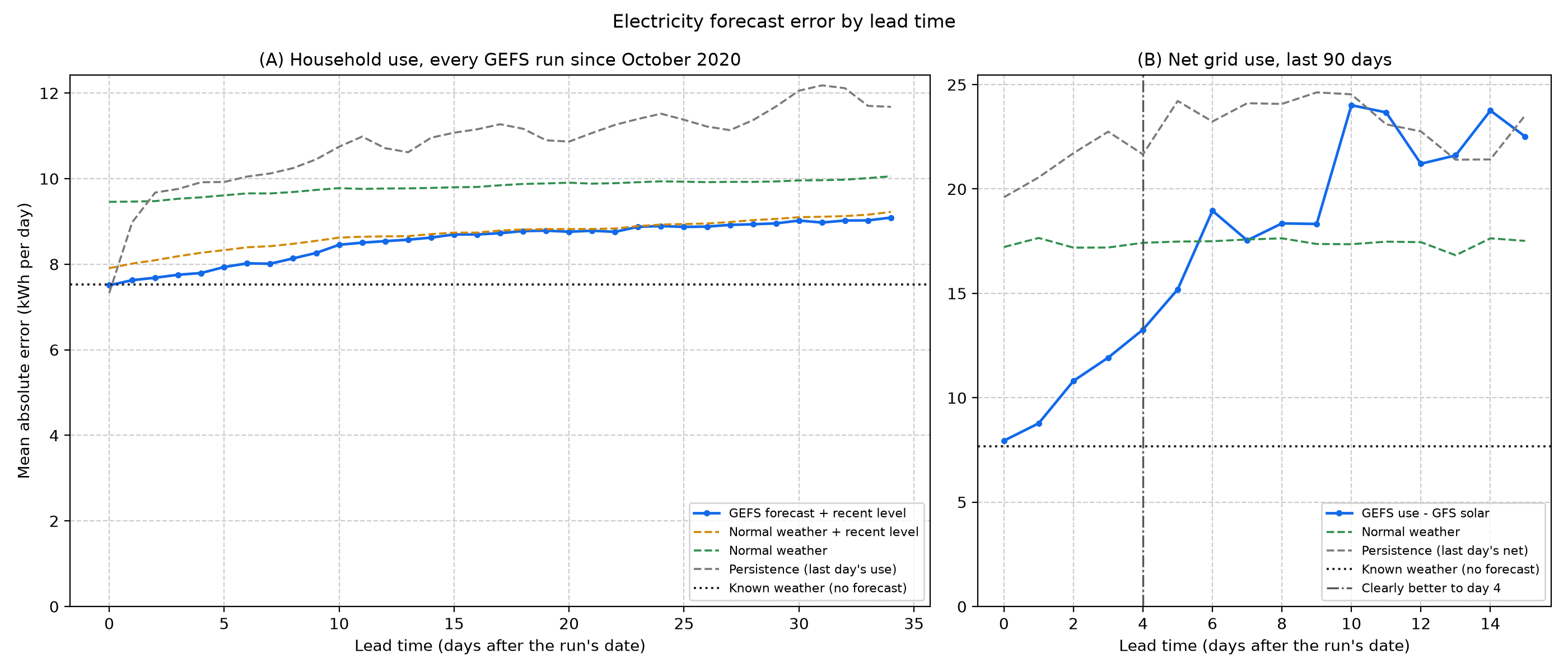
Figure 17. Electricity Forecast Error by Lead Time - (A) Every GEFS run since October 2020 replayed and scored against the use that followed. For tomorrow the forecast misses by 7.6 kWh on average, against 9.5 kWh for the normal, 9.0 kWh for repeating the last day and 8.0 kWh for the normal plus the recent level. At one week it misses by 8.0 kWh and at two weeks by 8.6 kWh. It beats the normal at every lead time out to five weeks. The gap between the forecast and the orange line (normal weather plus the recent level) is what the weather forecast itself adds: 0.4 kWh a day for tomorrow. Most of the gain over the plain normal comes from the recent level. For today, repeating yesterday (7.3 kWh) is as good as any model. With the actual temperature known (dotted) the error is still 7.5 kWh (9.1 kWh without the recent level): daily use is mostly habits. Weekly totals are steadier: for the coming week the forecast misses by 36 kWh of a typical 293 kWh (12%), against 51 kWh for the normal and 51 kWh for persistence. The 8-in-10 range held the actual day 83% of the time. (B) Net grid use since the solar forecasts began: tomorrow's net misses by 8.8 kWh, against 17.7 kWh for normal weather. Net use is clearly better than the normal (95% bootstrap interval of skill above zero) through day 4 and better on average through day 5, about as far as the solar forecast (Figure 13): beyond that, cloud cover is the larger unknown.

Station checks

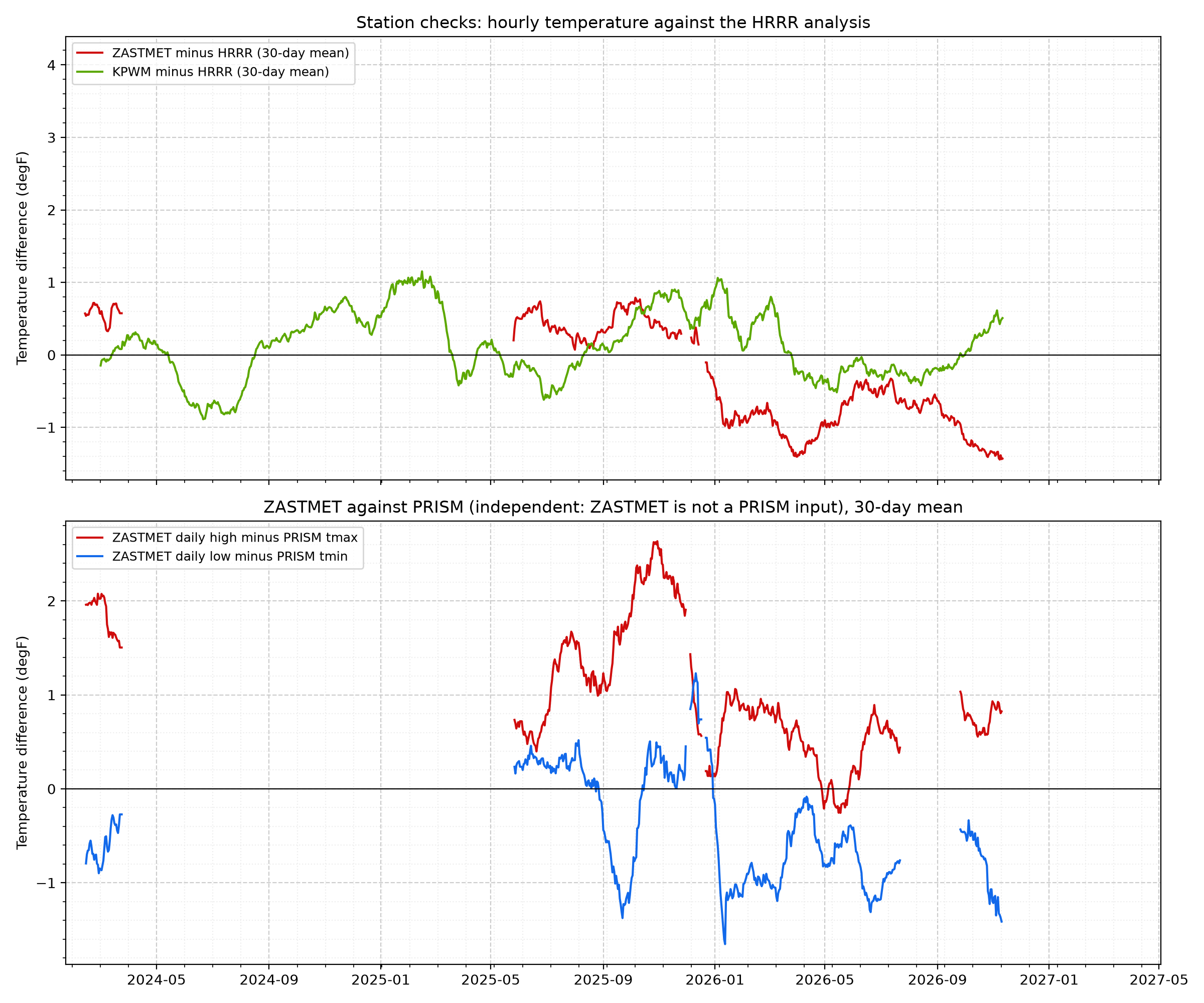
Figure 18. Station Checks Against Gridded References - Top: each station's hourly temperature minus the HRRR analysis at its grid cell, as a 30-day mean. Over the last year ZASTMET averaged -0.8 degF and KPWM +0.1 degF. A steady offset is expected (a 3 km grid cell is not a point); a sudden change in the offset points to a sensor or siting problem. HRRR assimilates KPWM, so KPWM agrees closely by design. Bottom: ZASTMET's daily high and low against PRISM, which does not use ZASTMET, over 515 days: highs average +1.0 degF and lows -0.4 degF relative to PRISM.

Data sources and credits

NOAA HRRR, GFS and GEFS data from NOAA NWS NCEP, processed by dynamical.org from NOAA Open Data Dissemination archives (CC BY 4.0).
PRISM Group, Oregon State University, https://prism.oregonstate.edu, daily data and 1991-2020 normals, accessed November 13, 2026.
House weather station (ZASTMET, Ambient Weather), Portland Jetport (KPWM, NWS), and SolarEdge production records from this project's database.

← Back to the main page.