Energy Analysis — Weather and Home Energy Use Near Cumberland Center, Maine
About This Section: These analyses apply statistical methods to understand how weather affects energy consumption. The house uses natural gas for heating (hydronic boiler system) and electricity for cooling (window/portable AC units, added over time). A hot tub has been in continuous use since June 2020 (inflatable June 2020-April 2021, Softub since April 2021).
Temperature Response and Load Profiles
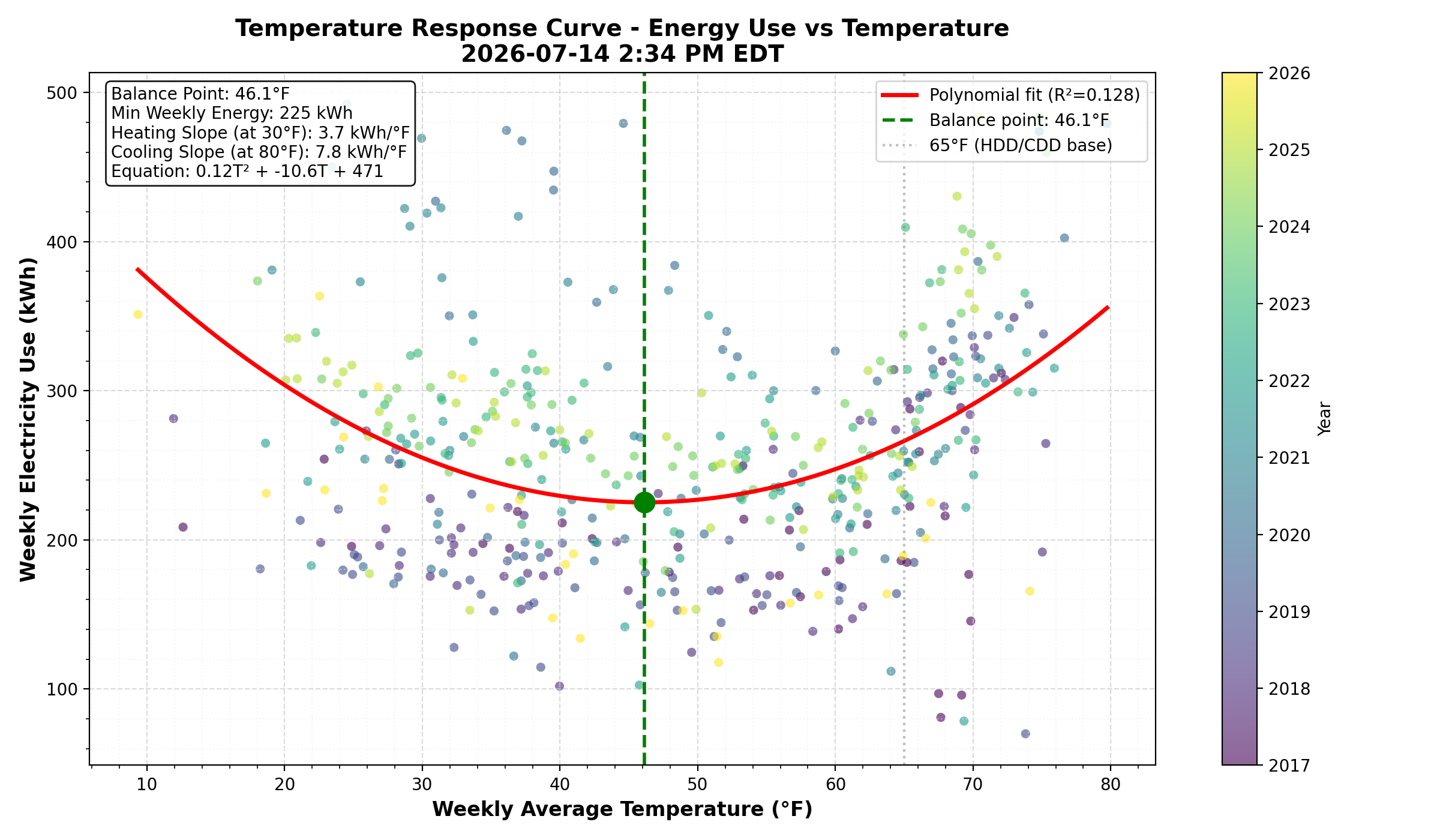
Figure 1. Temperature Response Curve - This polynomial regression shows the classic U-shaped relationship between outdoor temperature and electricity consumption. The balance point (minimum of the curve) identifies the temperature at which the building requires minimal heating or cooling. For this home, the balance point is around 46°F, lower than the typical 65°F baseline, suggesting good insulation or cooler temperature preferences. The steeper cooling slope (right arm) compared to heating slope indicates that AC systems are more energy-intensive than supplemental electric heating.
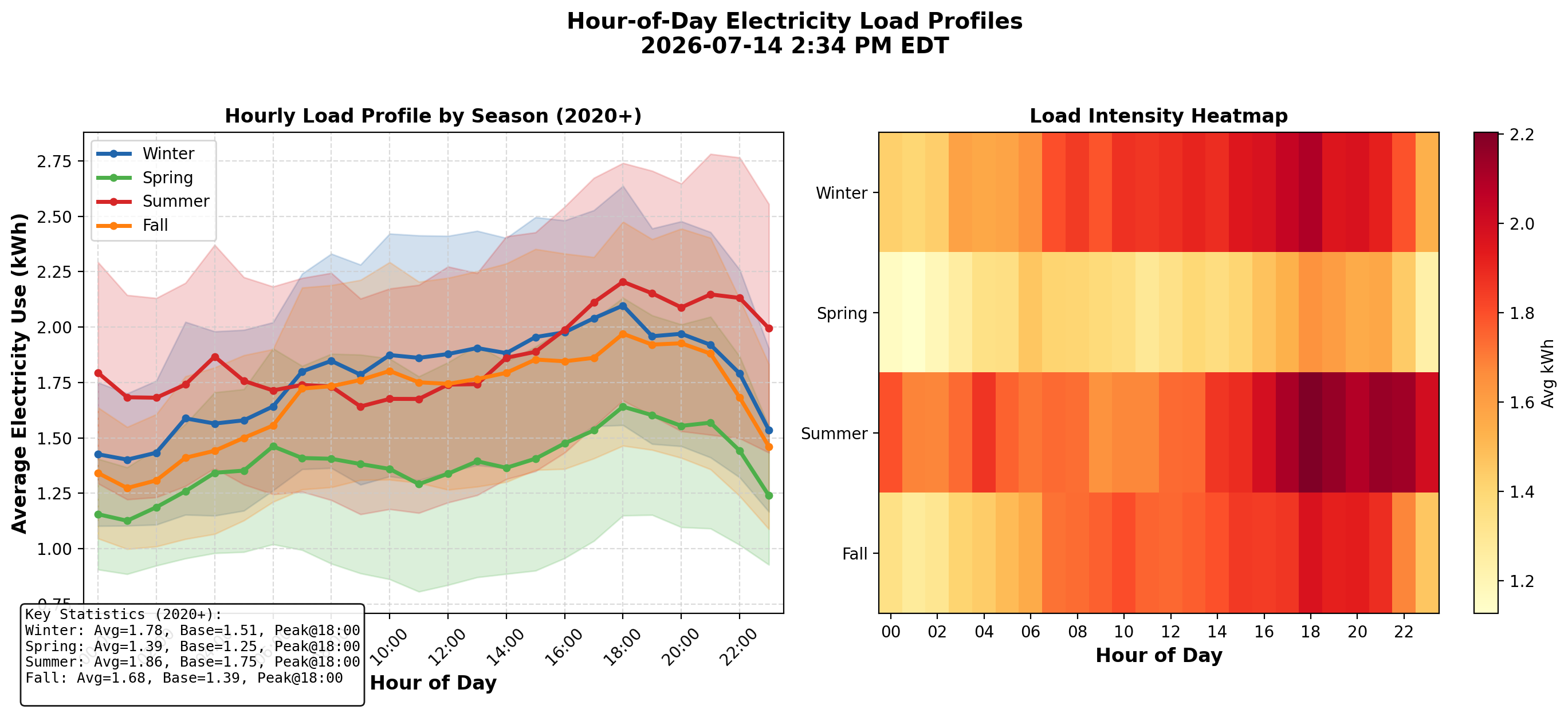
Figure 2. Hour-of-Day Load Profiles - This analysis reveals daily consumption patterns by season. Summer (red) shows the classic afternoon/evening peak from AC usage. Winter (blue) maintains elevated usage throughout the day from the hot tub and supplemental heating. The baseload (overnight 1am-5am average) represents always-on appliances like refrigerators, routers, and standby loads. Peak demand consistently occurs around 6pm across all seasons.
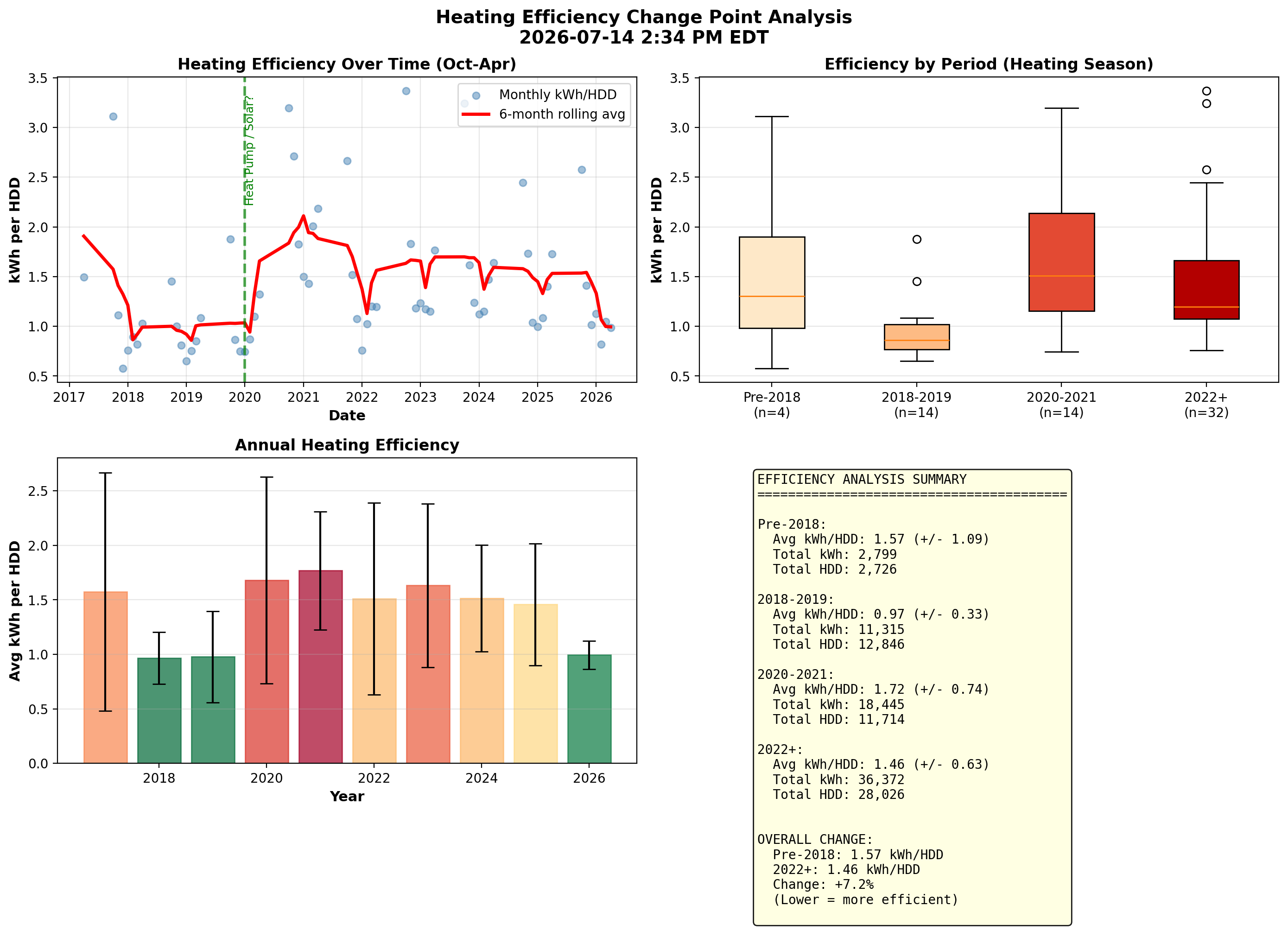
Figure 3. Efficiency Change Point Analysis - This tracks kWh per Heating Degree Day (HDD) over time to identify changes in heating efficiency. Lower values indicate better efficiency. The analysis breaks data into periods to detect the impact of equipment changes or behavioral shifts. Note: Primary heating is natural gas, so this primarily captures supplemental electric loads and the hot tub's contribution during heating season.
Summer Cooling Analysis
These analyses focus on summer cooling loads, which are entirely electric. Additional AC units have been added to the house over the years to improve comfort.
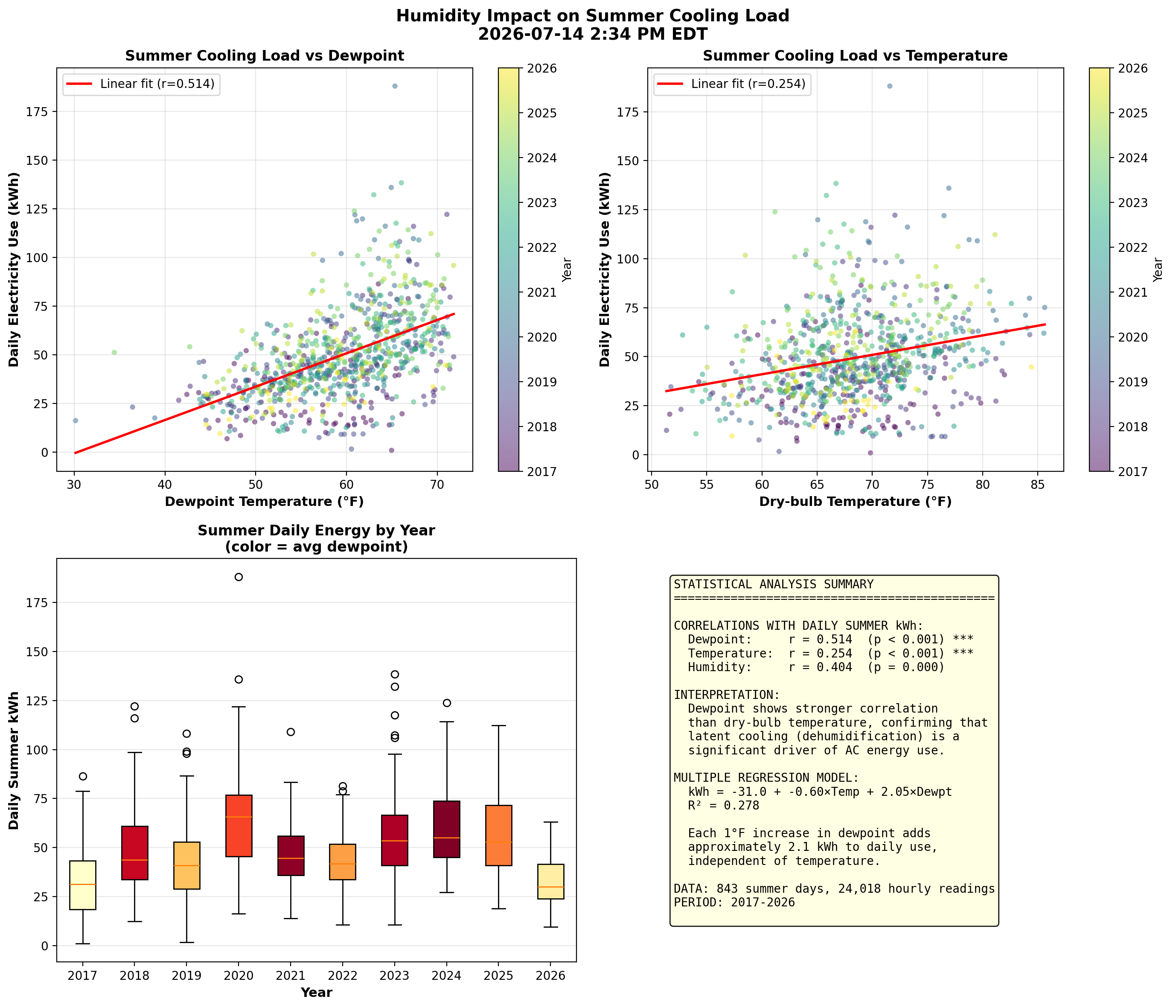
Figure 4. Humidity Impact on Cooling - Air conditioners must handle both sensible cooling (lowering temperature) and latent cooling (removing moisture). Dewpoint temperature directly measures air moisture content and often predicts AC energy use better than dry-bulb temperature alone. Statistical analysis shows dewpoint has a stronger correlation (r ≈ 0.51) with summer energy use than temperature (r ≈ 0.25). Each 1°F increase in dewpoint adds approximately 2 kWh to daily summer consumption, confirming that humid days drive higher AC loads due to dehumidification requirements.
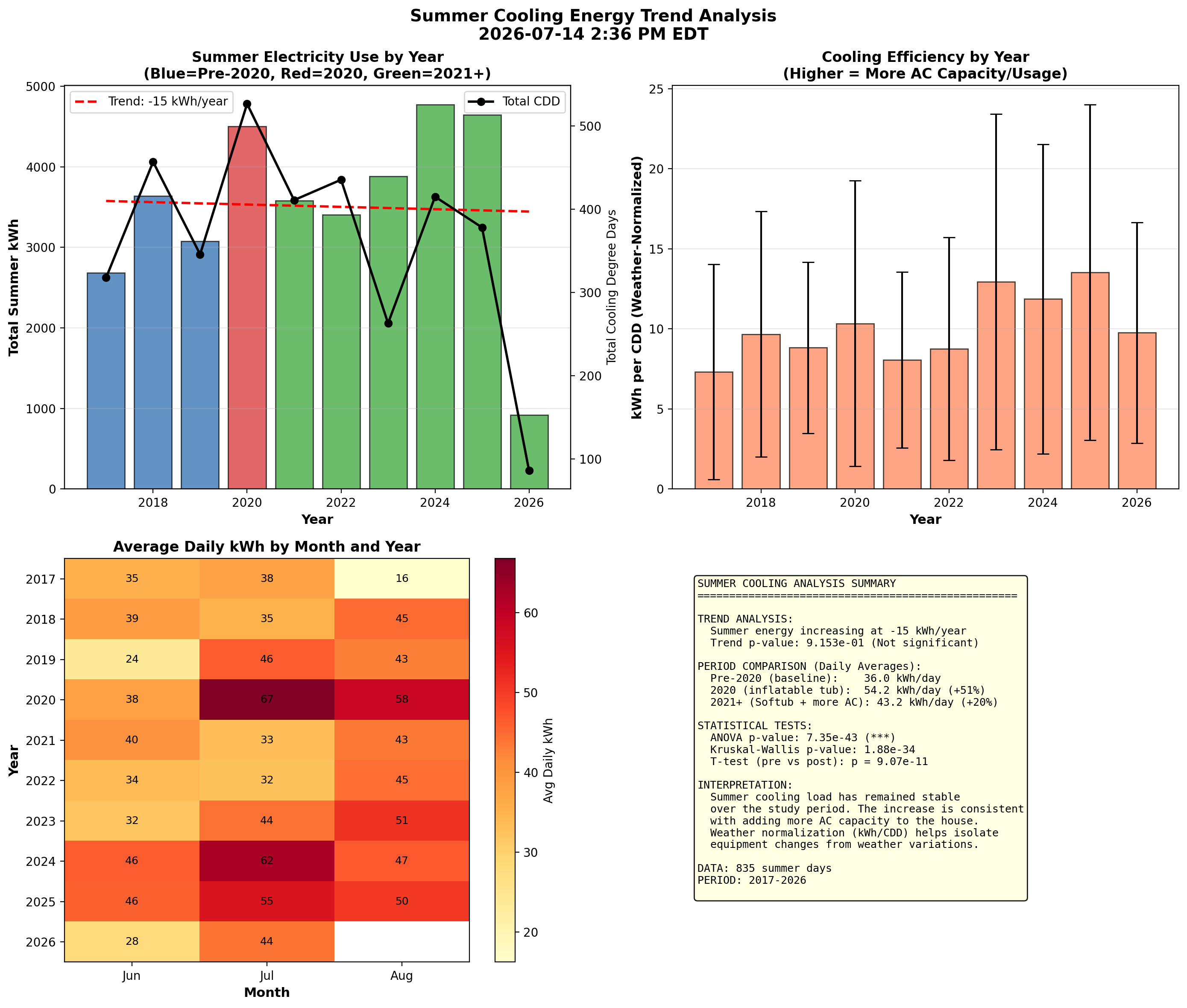
Figure 5. Summer Cooling Trend - This year-over-year analysis tracks summer electricity consumption normalized by Cooling Degree Days (CDD) to account for weather variations. Key findings:
- Pre-2020: Lower baseline (~36 kWh/day)
- 2020: Significant jump from inflatable hot tub (~54 kWh/day)
- 2021+: Settled to higher level with Softub + more AC capacity (~44 kWh/day)
Heating and Wind Effects
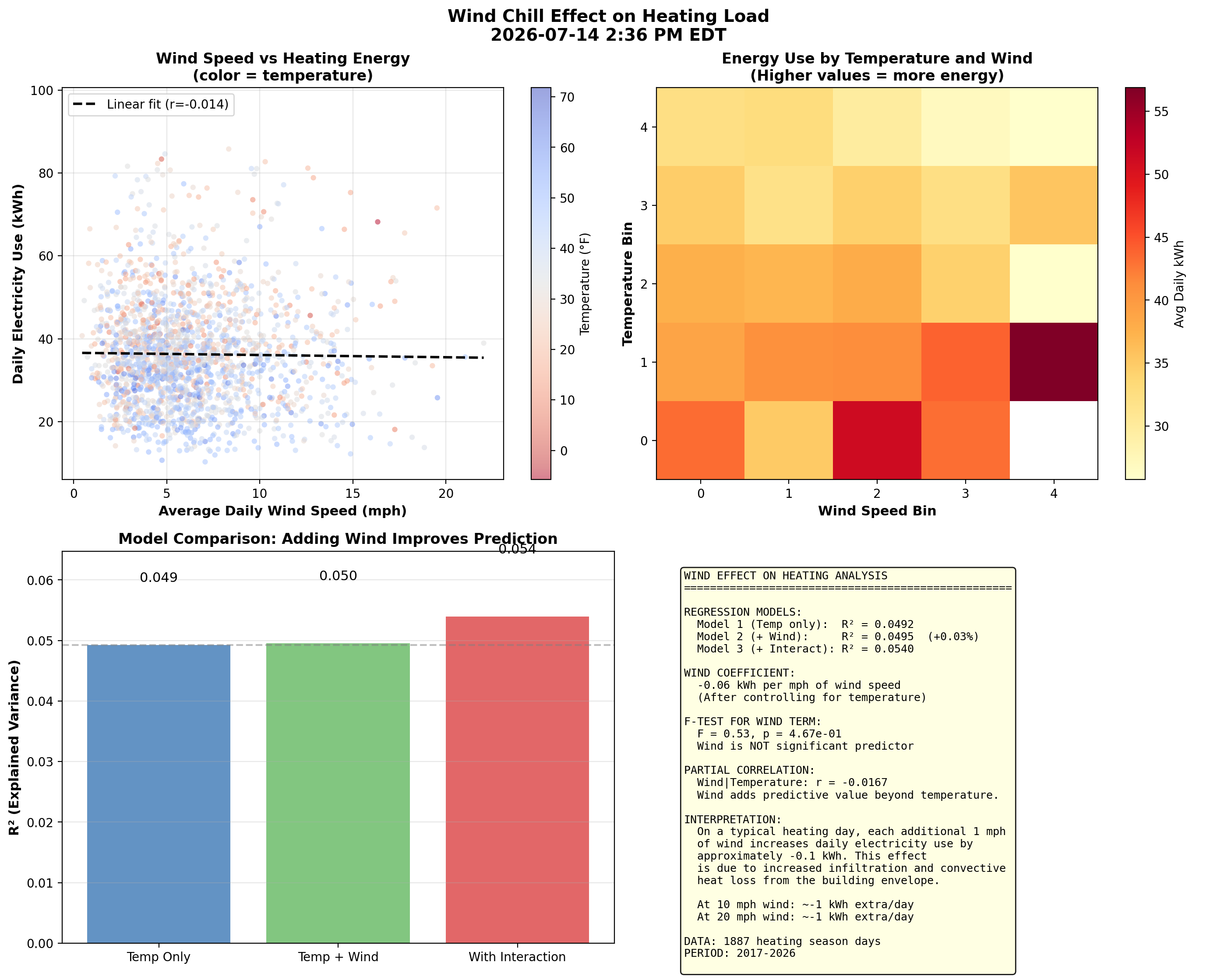
Figure 6. Wind Effect on Heating - Wind increases building heat loss through infiltration (cold air forced through gaps) and convection (faster heat transfer from exterior surfaces). This analysis tests whether wind speed adds predictive power beyond temperature alone. Results show wind has a small but measurable effect, with each additional mph of wind adding approximately 0.5 kWh per day at cold temperatures. The effect is most pronounced below 20°F where heating loads are highest. Note: Primary heating is natural gas; this analysis captures electric supplemental loads.
Weather Station Comparison
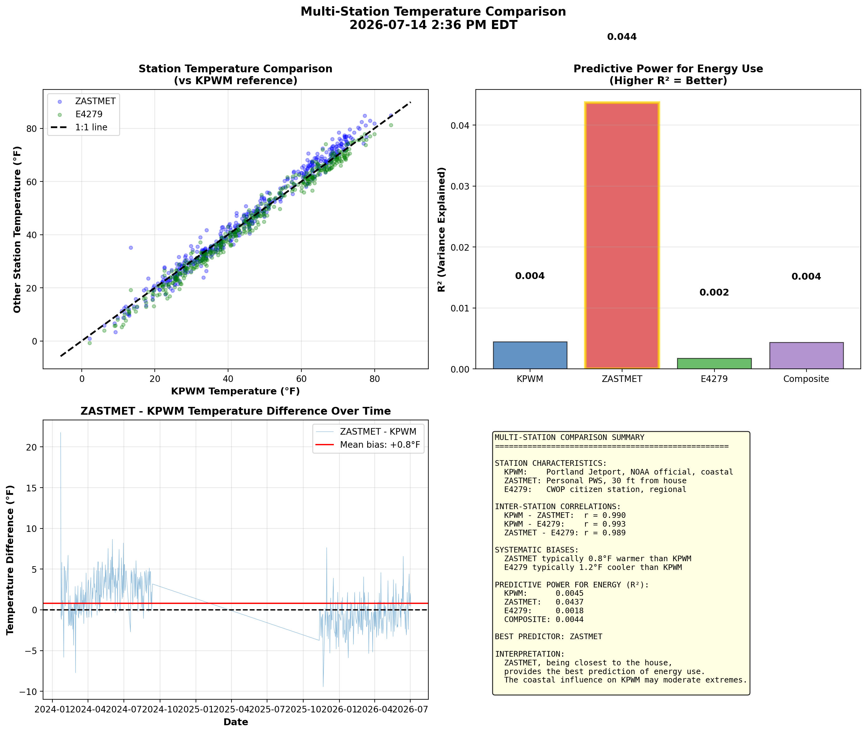
Figure 7. Multi-Station Temperature Comparison - This analysis compares three weather data sources:
- KPWM: Portland Jetport (official NOAA station, accurate but coastal, ~15 mi away)
- ZASTMET: Personal weather station 30 feet from the house
- E4279: Citizen Weather Observer Program station (closer than KPWM)
Energy Anomaly Detection
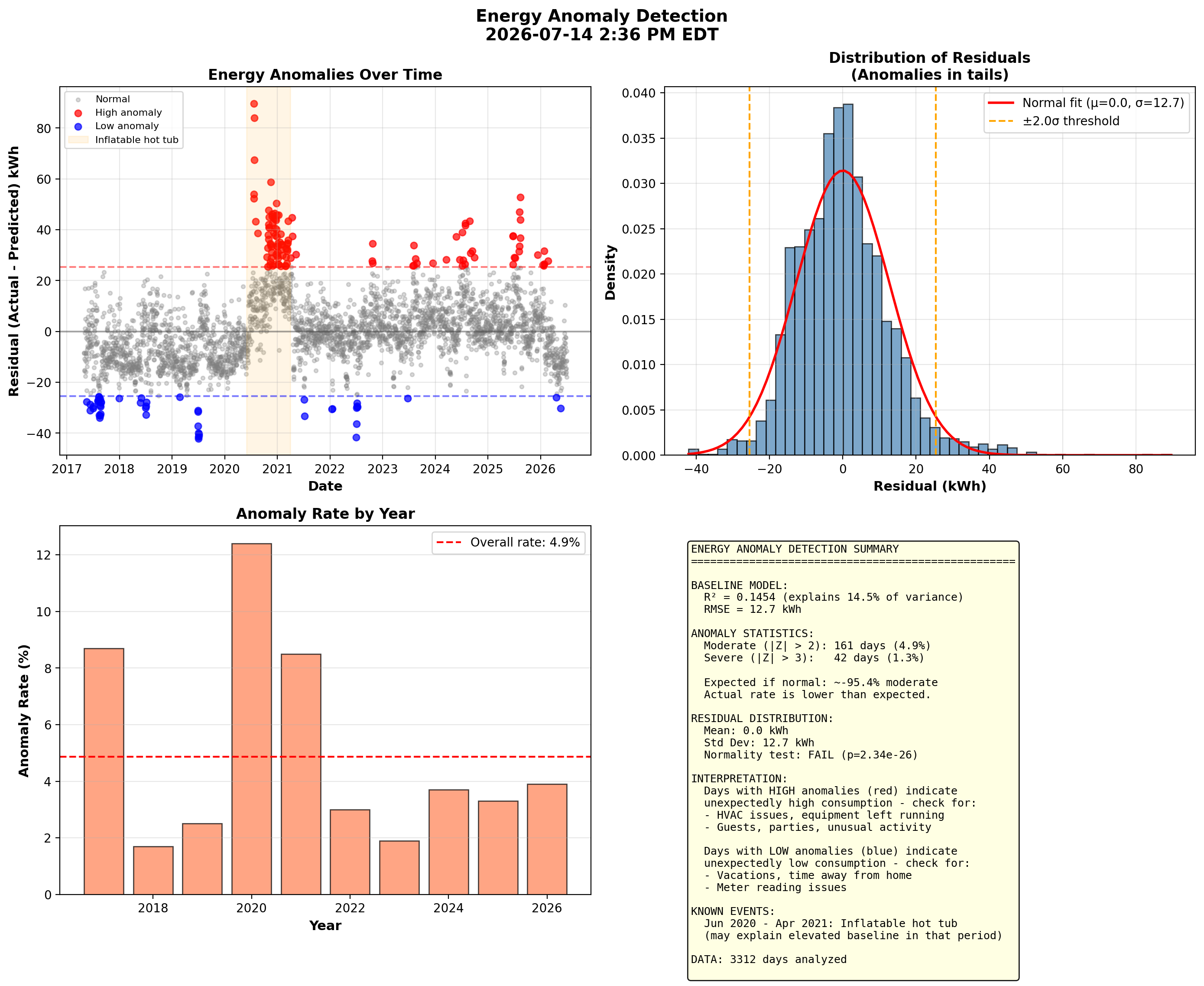
Figure 8. Energy Anomaly Detection - This analysis builds a baseline model predicting daily energy from temperature and identifies days that deviate significantly (beyond 2 standard deviations). High anomalies (red) may indicate equipment issues, guests, or unusual activity. Low anomalies (blue) often correspond to vacations or time away. The inflatable hot tub period (June 2020-April 2021) shows elevated residuals, confirming its significant energy impact. July 2020 contains several of the highest anomaly days, coinciding with hot tub break-in and summer heat.
Cost and Efficiency Metrics
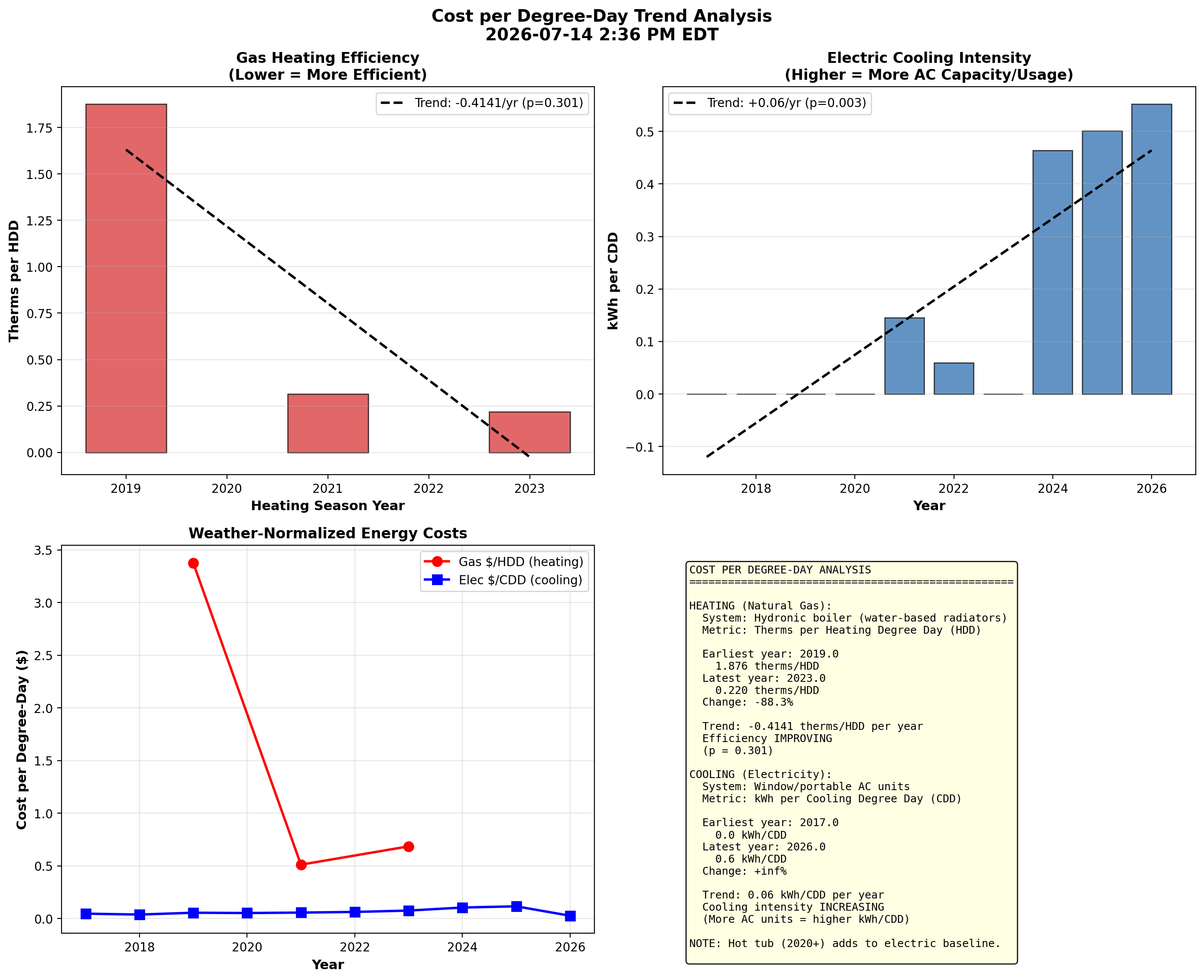
Figure 9. Cost per Degree-Day Trends - This weather-normalizes energy costs to track true efficiency over time:
- Gas heating (therms/HDD): Lower is better - shows heating system efficiency
- Electric cooling (kWh/CDD): Increasing values reflect added AC capacity, not inefficiency
Data Quality: Bill vs Meter Reconciliation
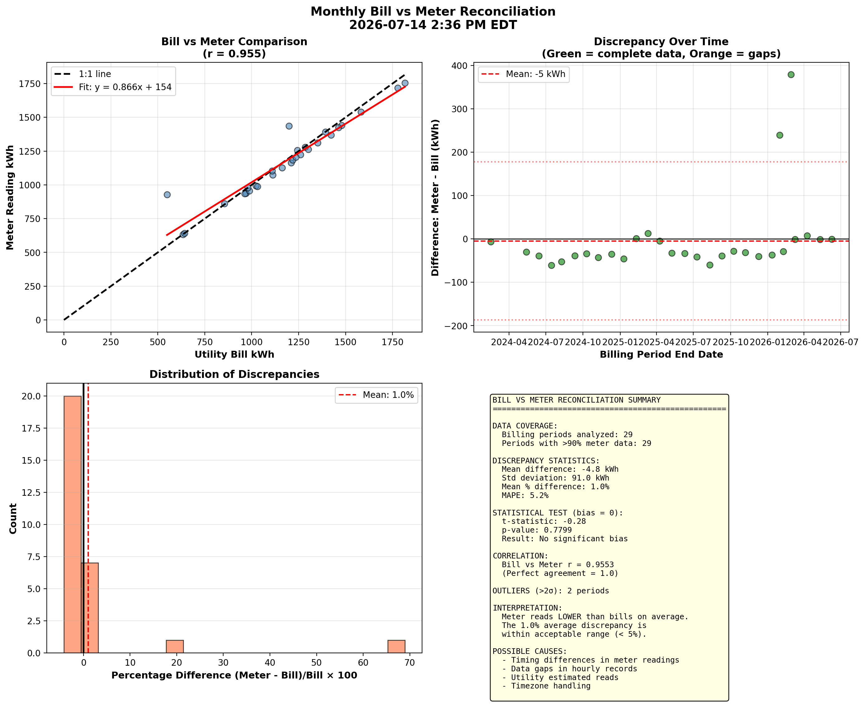
Figure 10. Bill vs Meter Reconciliation - This compares the smart meter's hourly readings (aggregated to billing periods) against utility bill kWh values. High correlation validates the meter data used throughout these analyses. Small discrepancies arise from timing differences, data gaps, and timezone handling. Periods with significant gaps in hourly data (shown in orange) are expected to show larger discrepancies.
View Net-Metering Reconciliation Report - A narrative assessment, rebuilt nightly, of whether CMP's net-metering credits match the revenue meter and the SolarEdge monitoring — including the dollar value of any gaps.
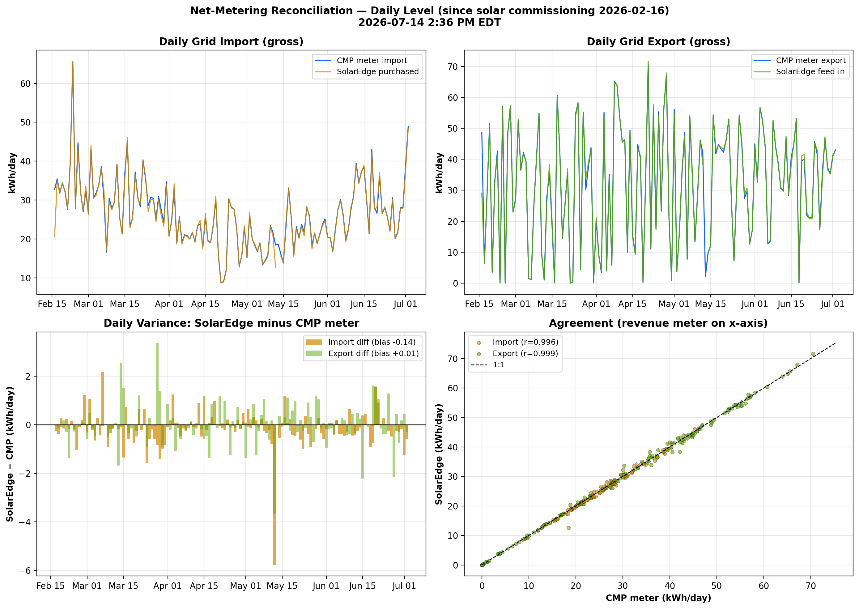
Figure 11. Net-Metering Reconciliation — Daily Level - Compares daily gross grid import and export between the CMP revenue meter (hourly interval data) and the SolarEdge monitoring system (15-minute CT-clamp data) since solar commissioning. The variance panel shows the daily difference between the two meters; the scatter shows overall agreement against the 1:1 line.
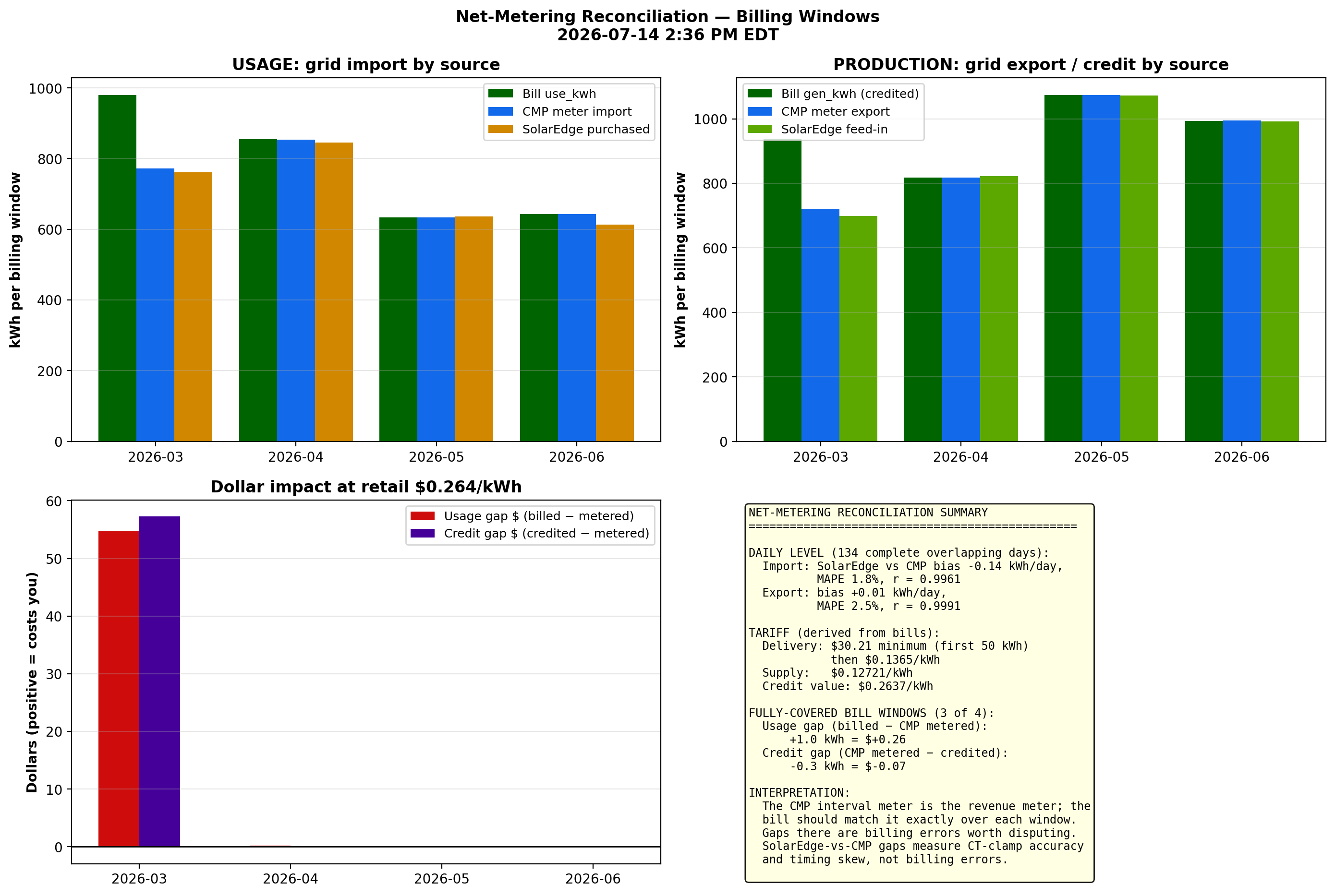
Figure 12. Net-Metering Reconciliation — Billing Windows - Rolls the two meters up into each CMP billing window and compares them against what the bill actually charged (usage) and credited (generation). The dollar panel prices any gap at the full retail rate (delivery volumetric + supply) that each net-metering credit kWh offsets, answering whether the credits are returning proper value.
Balance Point Shift Analysis
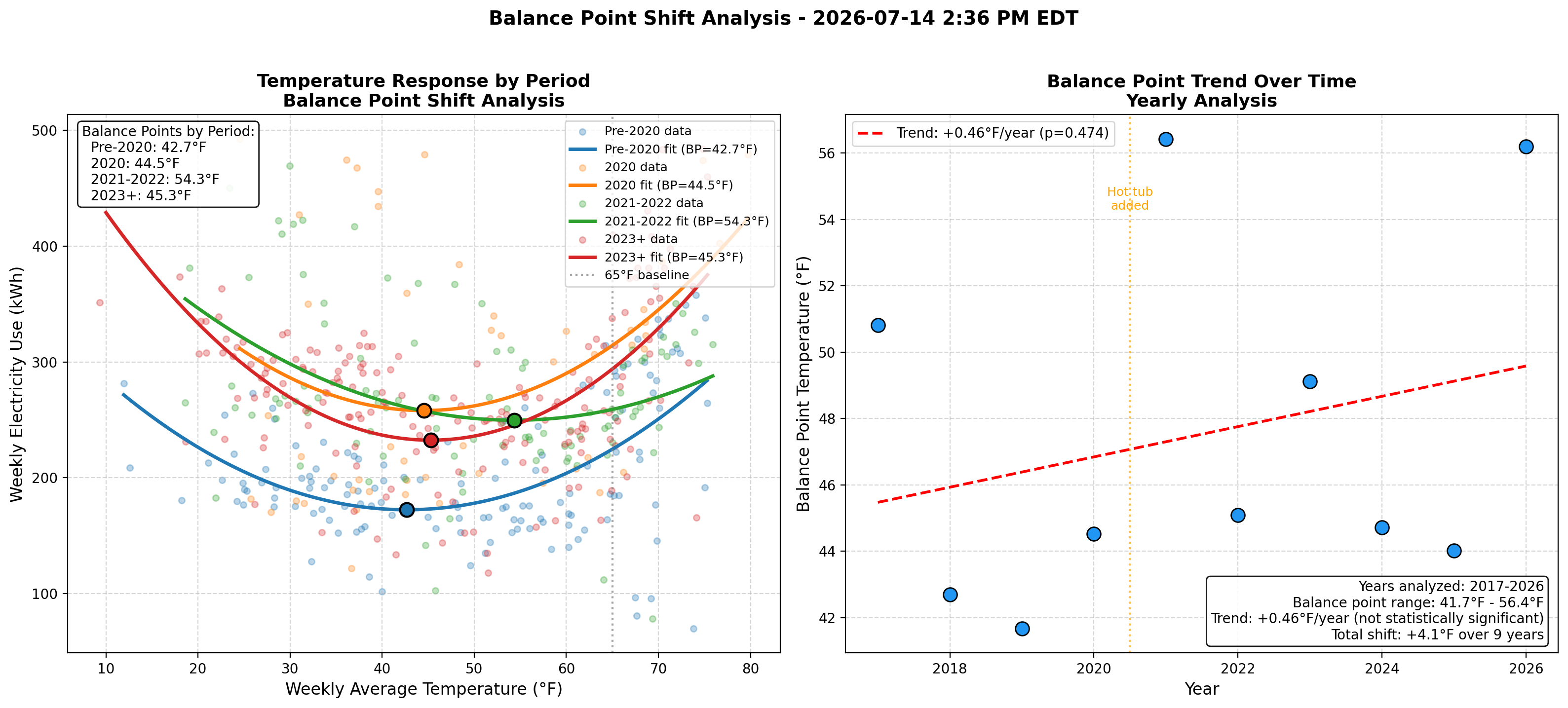
Figure 13. Balance Point Shift Over Time - This analysis examines whether the temperature "balance point" (the outdoor temperature at which energy use is minimized) has shifted over the years. The left panel shows temperature response curves fitted separately for different time periods, revealing how the U-shaped relationship between temperature and energy use has evolved. The right panel tracks yearly balance points to identify trends. Key findings:
- Pre-2020: Balance point ~42°F, indicating lower cooling loads
- 2020: Hot tub addition raised baseline but balance point similar (~44°F)
- 2021-2022: Balance point shifted to ~54°F, likely reflecting additional AC capacity
- 2023+: Balance point returned to ~45°F as usage patterns stabilized
Page Last modified: October 23, 2026