Temperatures Near Cumberland Center, Maine from Four Volunteer Meteorological Stations
Data provided graciously by https://weather.gladstonefamily.net
and the Citizen Weather Observer
Program. Also the NOAA National Weather Service.
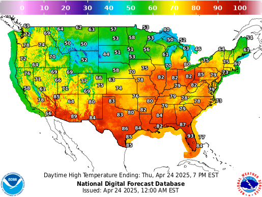
Other National maps. This one is Interactive
The source code for collecting data and generating charts is available on request. Charts are refreshed nightly.
Data Quality
View Data Quality Report - Monitor data freshness, completeness, range validation, energy trends, and seasonality patterns across all weather stations and energy data sources.
Temperature Charts

Figure 1. Weekly air temperatures for the previous 12 weeks at the four observation stations.
In all charts, Max Data is the latest measurement from the database. This Week, or this whatever time period, is the date the chart was generated.
Variance between the two indicates that either data for the current day is not available in the database for some reason (if This Week is later than Max Data) or someone went back in time and ran the chart scripts before the data were loaded (if This Week is earlier than Max Data).

Figure 2. Yearly comparison of weekly average air temperatures at station e4279

Figure 3. Yearly comparison of weekly average air temperatures at station KPWM

Figure 4. Comparison of a few years of temps for the last 30 days of daily temps for station KPWM agentically coded by Claude.ai
G-Series CWOP Stations
These are newer Citizen Weather Observer Program (CWOP) stations in the area, started in 2024-2025.
G5290 (Started Aug 2024)

Weekly average temps by week number |

60-day daily temperature comparison |
G5544 (Started Nov 2024)

Weekly average temps by week number |

60-day daily temperature comparison |
ZASTMET Real-Time Data

Figure 5. Last 48 hours of 5-minute data from the ZASTMET station. Made by both Copilot and Claude

Figure 6. Full record of 5-minute data from the ZASTMET station. Made by both Copilot and Claude

Figure 7. Wind conditions over the previous 24 hours at ZASTMET

Figure 8. Wind conditions over the previous 24 hours at KPWM
 Figure 9. KPWM Weekly temperature and electricity for the period of record |
 Figure 10. E4279 Weekly temperature and electricity for the period of record |

Figure 11. KPWM Daily temperature and electricity for the last 60 days
Updated cost per khw from .18 to .25 on April 4, 2023

Figure 12. Monthly gas and electricity use

Figure 13. Monthly gas and electricity cost in dollars

Figure 14. Annual gas and electricity cost in dollars

Figure 15. Monthly cumulative electricity use (30.4-day periods) from hourly meter data

Figure 16. Monthly cumulative electricity use (30.4-day periods) from hourly meter data for previous three years

Figure 17. Weekly electricity use against average temperature at KPWM before the year 2020

Figure 18. Weekly electricity use against weekly cumulative Heating Degree Days (HDD) using the 65 degree point at KPWM before the year 2020
From weather.gov
Degree days are based on the assumption that when the outside
temperature is 65°F, we don't need heating or cooling to be comfortable.
Degree days are the difference
between the daily temperature mean,
(high temperature plus low temperature divided by two) and 65°F. If the temperature mean is above 65°F, we
subtract 65 from the mean and
the result is Cooling Degree Days. If the temperature mean is below 65°F, we subtract the mean from 65 and the
result is Heating Degree Days.
days occur in the summer and occasionally in the fall

Figure 19. Weekly electricity use against average temperature at KPWM for the year 2020 and after

Figure 20. Weekly electricity use against weekly cumulative Heating Degree Days (HDD) using the 65 degree point at KPWM for the year 2020 and after

Figure 21. Annual energy costs by year. Also showing therms of heat applied through gas as normalizer for use.
Two different elevations for each station are shown in the table. Elevations from the US National Elevation Dataset appear to be the most accurate.

Figure 22. Monthly electricity costs for each kwh used as a scatter plot.
The entire electric bill is used to calculate cost. Therefore if the delivery costs go up, but the commodity (cost of each kwh from the supplier) stays the same, the apparent cost to deliver the electricity will still rise. This shows any possible relation between khws used and the cost per kwh.
Colors highlight the drift upward over time.

Figure 23. Monthly electricity dollars (cents) for each kwh over time.
The entire electric bill is used to calculate cost. Therefore if the delivery costs go up, but the commodity (cost of each kwh from the supplier) stays the same, the apparent cost to deliver the electricity will still rise.
This should show a rise over time of cost per kwh as delivered to the house, which incorporates both commodity as well as infrastructure/business cost changes.

Figure 24. Monthly cost per unit of energy delivered — electricity (left axis, $/kWh, blue) and natural gas (right axis, $/therm, red) over the full period of record. Electric data begins Nov 2015; gas data begins Dec 2016. Both series use actual billed totals divided by metered consumption from v_monthly_utilities_better. Dual axes are needed because the two units are not directly comparable: 1 therm = 100,000 BTU, while 1 kWh ≈ 3,412 BTU.

Figure 25. Annual average cost per unit of energy delivered — electricity (left axis, $/kWh, blue bars) and natural gas (right axis, $/therm, red bars), aggregated from the monthly data shown in Figure 24. Error bars span the full monthly min–max range within each year, reflecting seasonal rate variation. Dashed lines show the linear trend for each series over the period of record. * Current year is partial (year-to-date only).
Energy Analysis
About This Section: These analyses apply statistical methods to understand how weather affects energy consumption. The house uses natural gas for heating (hydronic boiler system) and electricity for cooling (window/portable AC units, added over time). A hot tub has been in continuous use since June 2020 (inflatable June 2020-April 2021, Softub since April 2021).
Temperature Response and Load Profiles

Figure 26. Temperature Response Curve - This polynomial regression shows the classic U-shaped relationship between outdoor temperature and electricity consumption. The balance point (minimum of the curve) identifies the temperature at which the building requires minimal heating or cooling. For this home, the balance point is around 46°F, lower than the typical 65°F baseline, suggesting good insulation or cooler temperature preferences. The steeper cooling slope (right arm) compared to heating slope indicates that AC systems are more energy-intensive than supplemental electric heating.

Figure 27. Hour-of-Day Load Profiles - This analysis reveals daily consumption patterns by season. Summer (red) shows the classic afternoon/evening peak from AC usage. Winter (blue) maintains elevated usage throughout the day from the hot tub and supplemental heating. The baseload (overnight 1am-5am average) represents always-on appliances like refrigerators, routers, and standby loads. Peak demand consistently occurs around 6pm across all seasons.

Figure 28. Efficiency Change Point Analysis - This tracks kWh per Heating Degree Day (HDD) over time to identify changes in heating efficiency. Lower values indicate better efficiency. The analysis breaks data into periods to detect the impact of equipment changes or behavioral shifts. Note: Primary heating is natural gas, so this primarily captures supplemental electric loads and the hot tub's contribution during heating season.
Summer Cooling Analysis
These analyses focus on summer cooling loads, which are entirely electric. Additional AC units have been added to the house over the years to improve comfort.

Figure 29. Humidity Impact on Cooling - Air conditioners must handle both sensible cooling (lowering temperature) and latent cooling (removing moisture). Dewpoint temperature directly measures air moisture content and often predicts AC energy use better than dry-bulb temperature alone. Statistical analysis shows dewpoint has a stronger correlation (r ≈ 0.51) with summer energy use than temperature (r ≈ 0.25). Each 1°F increase in dewpoint adds approximately 2 kWh to daily summer consumption, confirming that humid days drive higher AC loads due to dehumidification requirements.

Figure 30. Summer Cooling Trend - This year-over-year analysis tracks summer electricity consumption normalized by Cooling Degree Days (CDD) to account for weather variations. Key findings:
- Pre-2020: Lower baseline (~36 kWh/day)
- 2020: Significant jump from inflatable hot tub (~54 kWh/day)
- 2021+: Settled to higher level with Softub + more AC capacity (~44 kWh/day)
Heating and Wind Effects

Figure 31. Wind Effect on Heating - Wind increases building heat loss through infiltration (cold air forced through gaps) and convection (faster heat transfer from exterior surfaces). This analysis tests whether wind speed adds predictive power beyond temperature alone. Results show wind has a small but measurable effect, with each additional mph of wind adding approximately 0.5 kWh per day at cold temperatures. The effect is most pronounced below 20°F where heating loads are highest. Note: Primary heating is natural gas; this analysis captures electric supplemental loads.
Weather Station Comparison

Figure 32. Multi-Station Temperature Comparison - This analysis compares three weather data sources:
- KPWM: Portland Jetport (official NOAA station, accurate but coastal, ~15 mi away)
- ZASTMET: Personal weather station 30 feet from the house
- E4279: Citizen Weather Observer Program station (closer than KPWM)
Energy Anomaly Detection

Figure 33. Energy Anomaly Detection - This analysis builds a baseline model predicting daily energy from temperature and identifies days that deviate significantly (beyond 2 standard deviations). High anomalies (red) may indicate equipment issues, guests, or unusual activity. Low anomalies (blue) often correspond to vacations or time away. The inflatable hot tub period (June 2020-April 2021) shows elevated residuals, confirming its significant energy impact. July 2020 contains several of the highest anomaly days, coinciding with hot tub break-in and summer heat.
Cost and Efficiency Metrics

Figure 34. Cost per Degree-Day Trends - This weather-normalizes energy costs to track true efficiency over time:
- Gas heating (therms/HDD): Lower is better - shows heating system efficiency
- Electric cooling (kWh/CDD): Increasing values reflect added AC capacity, not inefficiency
Data Quality: Bill vs Meter Reconciliation

Figure 35. Bill vs Meter Reconciliation - This compares the smart meter's hourly readings (aggregated to billing periods) against utility bill kWh values. High correlation validates the meter data used throughout these analyses. Small discrepancies arise from timing differences, data gaps, and timezone handling. Periods with significant gaps in hourly data (shown in orange) are expected to show larger discrepancies.
View Net-Metering Reconciliation Report - A narrative assessment, rebuilt nightly, of whether CMP's net-metering credits match the revenue meter and the SolarEdge monitoring — including the dollar value of any gaps.

Figure 36. Net-Metering Reconciliation — Daily Level - Compares daily gross grid import and export between the CMP revenue meter (hourly interval data) and the SolarEdge monitoring system (15-minute CT-clamp data) since solar commissioning. The variance panel shows the daily difference between the two meters; the scatter shows overall agreement against the 1:1 line.

Figure 37. Net-Metering Reconciliation — Billing Windows - Rolls the two meters up into each CMP billing window and compares them against what the bill actually charged (usage) and credited (generation). The dollar panel prices any gap at the full retail rate (delivery volumetric + supply) that each net-metering credit kWh offsets, answering whether the credits are returning proper value.
Balance Point Shift Analysis

Figure 38. Balance Point Shift Over Time - This analysis examines whether the temperature "balance point" (the outdoor temperature at which energy use is minimized) has shifted over the years. The left panel shows temperature response curves fitted separately for different time periods, revealing how the U-shaped relationship between temperature and energy use has evolved. The right panel tracks yearly balance points to identify trends. Key findings:
- Pre-2020: Balance point ~42°F, indicating lower cooling loads
- 2020: Hot tub addition raised baseline but balance point similar (~44°F)
- 2021-2022: Balance point shifted to ~54°F, likely reflecting additional AC capacity
- 2023+: Balance point returned to ~45°F as usage patterns stabilized
Residential Solar
Installed system (January 2026): 12.18 kW DC — 29 × REC420AA Pure 2 heterojunction modules (420 W, 21.7% efficiency, −0.24%/°C) with a per-module SolarEdge S440 optimizer, feeding a SolarEdge SE11400H-US Home Hub inverter (11.4 kW AC, 99% CEC efficiency, DC/AC ratio 1.07). Roof-mounted at tilt 37°, azimuth 215° (WSW). Grid-tied and net-metered with CMP; no battery (inverter is storage-ready). Module warranty 25 yr at 0.25%/yr degradation. Monitoring is revenue-grade, reporting to SolarEdge every 15 minutes.
Modeled expectations: two independent unshaded models agree within 1.3% — the installer design estimate (15,441 kWh/yr) and a PVGIS-5 run at the exact roof geometry (15,649 kWh/yr, ≈1,285 kWh/kWp). The steep 37° tilt flattens seasonality (July only ~1.9× December), which suits this home's winter heat-pump load. Tree shading and snow are not in these models; the design-vs-actual analysis below measures the real-world correction from monitoring data continuously and re-projects the current year and the 25-year outlook from it.
The charts below show how solar energy flows through the home: production is split between direct home use ("To Home") and export to the grid ("To Grid"), while consumption shows what comes from solar versus grid import.
Daily Energy Summary

Figure 39. Daily Energy Bars - Horizontal stacked bars showing today's energy breakdown. Production shows solar energy generated, split into power used directly by the home (green) and exported to the grid (blue). Consumption shows total home energy use, split between solar-sourced (light blue) and grid-imported (orange).
Daily Power Flow

Figure 40. Daily Site Power - 15-minute resolution power flow throughout the day. Production appears above the zero line, consumption below. The overlap of "To Home" and "From Solar" represents self-consumed solar energy. Peak production typically occurs around solar noon; morning and evening grid imports cover demand when solar production is insufficient.
Weekly Energy Summary

Figure 41. Weekly Energy Bars - Daily production and consumption totals for the past week. Day-to-day variation reflects weather conditions (cloud cover reduces production) and household activity patterns. The stacked colors show the breakdown between self-consumption, grid export, and grid import.
Weekly Power Flow

Figure 42. Weekly Site Power - Seven days of 15-minute power data showing the daily solar generation pattern. Clear days show smooth bell curves; cloudy days show irregular production. This view helps identify weather impacts and consumption patterns over the week.
Net Energy Balance

Figure 43. Weekly Net Energy - Daily net energy balance (production minus consumption). Blue bars above zero indicate days when solar production exceeded household consumption (surplus exported to grid). Orange bars below zero indicate days when consumption exceeded production (deficit imported from grid). This view quickly shows whether the home is a net producer or consumer on any given day.

Figure 44. Monthly Net Energy - Monthly net energy balance showing the cumulative effect over longer periods. Positive months (blue) indicate net energy export to the grid; negative months (orange) indicate net grid import. Over a full year, this chart will reveal seasonal patterns - expect surpluses in sunny months and deficits in winter when days are shorter and heating loads higher.
Monthly Energy Summary

Figure 45. Monthly Energy Bars - Monthly production and consumption totals for all available data, using the same side-by-side stacked bar layout as the weekly chart (Figure 41). Each month shows two bars: Production (left) split between energy used directly by the home (green) and exported to the grid (blue); Consumption (right) split between solar-sourced (light blue) and grid-imported (orange). Seasonal patterns are clearly visible — summer months show high production with significant grid export, while winter months show lower production and heavier grid import to meet household demand.
Design vs. Actual Production
View Solar Design-vs-Actual Report - A narrative assessment, rebuilt nightly, of how measured production compares to the PVGIS design model month by month, the learned real-world correction factor, and continuously re-adjusted projections for the current year and the 25-year system life.

Figure 46. Modeled vs. Actual Monthly Production - Monthly SolarEdge production measured against the unshaded PVGIS design model. The ratio panel tracks actual/model by month; the learned correction factor (production-weighted over complete months) turns the unshaded model into a measured real-world expectation, absorbing tree shading, snow, and weather in one number that sharpens as months accumulate.

Figure 47. Adjusted Production Outlook - The current year assembled from measured months plus correction-adjusted model for the remainder, then projected across the 25-year module warranty life at 0.25%/yr degradation. Shown against the unshaded model ceiling and the installer design estimate for context.
Will Solar Cover the House?
Bottom line: measured to date, the system can deliver this household's annual electricity needs. The house uses about 14,731 kWh per year (average of 2021–2025); the array's measurement-adjusted output is 15,556 kWh per full year — 106% of annual needs.
Panel aging (0.25%/yr) erodes this slowly: coverage stays above 100% until 2048, ending the 25-year warranty life at 99%.
For 2026 itself (a partial year — commissioned January 28), estimated production of 14,804 kWh covers 100% of the needs baseline. Consumption is currently pacing 17,205 kWh/yr (above the historical average — watch this: rising use shrinks coverage).
Coverage is an annual statement, not a monthly one: so far in 2026 the house was a net exporter in April, May, June and a net importer the other months. Under CMP net-energy billing the summer surplus banks as credits (12-month rolling) that pay down winter deficits — which is why the annual number is the one that matters.
Recomputed 2026-07-14 2:37 PM EDT from SolarEdge monitoring, the CMP interval meter, and the PVGIS design model (correction factor 0.994, 5 complete months). Method and detail: Solar Design-vs-Actual Report.

Figure 48. Rooftop solar array configuration at the home base. The 12.18 kW system whose production data is tracked throughout this page.
stations
Layers
Figure 49. Interactive map served from weathermap.fluidgrid.site via MapLibre GL and PMTiles

Figure 50. Plumbing. This is how this site is maintained.
- Data is stored in a Maria DB database (fomerly MySQL) with a ton of views for easy data extraction and concise, centralized aggregation.
- Data shuffling logic is done with BASH shell scripts and the presentation (charts) is performed with matplotlib glued to the database through sqlalchemy, pandas, and numpy -- all Python libraries.
- Data operations all run on a Raspberry Pi 3B in the basement. The page and image you see are all static from a shared host and are updated nightly by jobs from the Pi.

Figure 51. A naked Raspberry Pi 3B

Figure 52. The Pi in action. USB-powered and connected over WiFi.
Page Last modified: July 14, 2026